Click here to download this notebook.

How to use a xarray Dataset as NadirData source

NadirData can be created using anything than can be opened as a xarray dataset and compute statistics on it in the exact same manner. It allows to dynamically create a dataset by using as many inputs as you want, align their coordinates if needed, arrange them however you want and use it has your data source [doc].

Example: JASON 3 - 20hz netCDF

import xarray as xr

from casys import NadirData, CasysPlot, Field, PlotParams

NadirData.enable_loginfo()

Create your source xarray dataset

# Open with xarray the product files of Jason-3 (Track 1 to 9 of cycle 127)
ds = xr.open_mfdataset(
    "/data/OCTANT_NG/cvi/JA3/JA3_GPN_2PdP127_00*.nc", combine="by_coords"
)

ds["alt_echo_type"]

<xarray.DataArray 'alt_echo_type' (time: 30130)> Size: 121kB
dask.array<concatenate, shape=(30130,), dtype=float32, chunksize=(3432,), chunktype=numpy.ndarray>
Coordinates:
  * time     (time) datetime64[ns] 241kB 2019-07-20T19:23:06.823509248 ... 20...
    lat      (time) float64 241kB dask.array<chunksize=(3411,), meta=np.ndarray>
    lon      (time) float64 241kB dask.array<chunksize=(3411,), meta=np.ndarray>
Attributes:
    long_name:      altimeter echo type
    flag_values:    [0 1]
    flag_meanings:  ocean_like non_ocean_like
    comment:        The altimeter echo type is determined by testing the rms ...

xarray.DataArray

'alt_echo_type'

• time: 30130

• dask.array<chunksize=(3411,), meta=np.ndarray>

  Array Chunk Bytes 117.70 kiB 13.41 kiB Shape (30130,) (3432,) Dask graph 9 chunks in 19 graph layers Data type float32 numpy.ndarray

• Coordinates: (3)
  • time
    (time)
    datetime64[ns]
    2019-07-20T19:23:06.823509248 .....

    long_name :

    time (sec. since 2000-01-01)

    standard_name :

    time

    tai_utc_difference :

    -37.0

    leap_second :

    0000-00-00 00:00:00

    comment :

    [tai_utc_difference] is the difference between TAI and UTC reference time (seconds) for the first measurement of the data set. [leap_second] is the UTC time at which a leap second occurs in the data set, if any. After this UTC time, the [tai_utc_difference] is increased by 1 second

    array(['2019-07-20T19:23:06.823509248', '2019-07-20T19:23:07.842218880',
           '2019-07-20T19:23:08.860929024', ..., '2019-07-21T03:48:59.781951872',
           '2019-07-21T03:49:00.800662016', '2019-07-21T03:49:01.819372160'],
          dtype='datetime64[ns]')

  • lat
    (time)
    float64
    dask.array<chunksize=(3411,), meta=np.ndarray>

    long_name :

    latitude

    standard_name :

    latitude

    units :

    degrees_north

    quality_flag :

    orb_state_flag_rest or orb_state_flag_diode

    comment :

    Positive latitude is North latitude, negative latitude is South latitude. See Jason-3 User Handbook. Associated quality flag is orb_state_flag_diode for the OGDR products, orb_state_flag_rest for the IGDR and GDR products

    Array Chunk Bytes 235.39 kiB 26.81 kiB Shape (30130,) (3432,) Dask graph 9 chunks in 19 graph layers Data type float64 numpy.ndarray

  • lon
    (time)
    float64
    dask.array<chunksize=(3411,), meta=np.ndarray>

    long_name :

    longitude

    standard_name :

    longitude

    units :

    degrees_east

    quality_flag :

    orb_state_flag_rest or orb_state_flag_diode

    comment :

    East longitude relative to Greenwich meridian. See Jason-3 User Handbook. Associated quality flag is orb_state_flag_diode for the OGDR products, orb_state_flag_rest for the IGDR and GDR products

    Array Chunk Bytes 235.39 kiB 26.81 kiB Shape (30130,) (3432,) Dask graph 9 chunks in 19 graph layers Data type float64 numpy.ndarray

• Indexes: (1)
  • time
    PandasIndex

    PandasIndex(DatetimeIndex(['2019-07-20 19:23:06.823509248',
                   '2019-07-20 19:23:07.842218880',
                   '2019-07-20 19:23:08.860929024',
                   '2019-07-20 19:23:09.879636736',
                   '2019-07-20 19:23:10.898348800',
                   '2019-07-20 19:23:11.917057024',
                   '2019-07-20 19:23:12.935769088',
                   '2019-07-20 19:23:13.954476800',
                   '2019-07-20 19:23:14.973187968',
                   '2019-07-20 19:23:15.991898112',
                   ...
                   '2019-07-21 03:48:53.594016128',
                   '2019-07-21 03:48:54.612728064',
                   '2019-07-21 03:48:55.631436800',
                   '2019-07-21 03:48:56.650147968',
                   '2019-07-21 03:48:57.203162240',
                   '2019-07-21 03:48:57.744533120',
                   '2019-07-21 03:48:58.763243136',
                   '2019-07-21 03:48:59.781951872',
                   '2019-07-21 03:49:00.800662016',
                   '2019-07-21 03:49:01.819372160'],
                  dtype='datetime64[ns]', name='time', length=30130, freq=None))

• Attributes: (4)

  long_name :

  altimeter echo type

  flag_values :

  [0 1]

  flag_meanings :

  ocean_like non_ocean_like

  comment :

  The altimeter echo type is determined by testing the rms of the high rate range measurements against a threshold as well as the number of valid high rate range measurements against a minimum value

Create your NadirData

# Create your NadirData object

selection = "is_bounded(-40, deg_normalize(-90, lat_20hz), 60) && is_bounded(-50, deg_normalize(-180, lon_20hz), 150)"

cd_ncdf = NadirData(
    source=ds,
    select_clip=selection,
    time="time_20hz",
    longitude="lon_20hz",
    latitude="lat_20hz",
)

cd_ncdf.show_fields(containing="swh_20hz")

Name	Description	Unit
swh_20hz_ku	20 Hz Ku band corrected significant waveheight All instrumental corrections included, i.e. modeled instrumental errors correction (modeled_instr_corr_swh_ku) and system bias	m
swh_20hz_c	20 Hz C band corrected significant waveheight All instrumental corrections included, i.e. modeled instrumental errors correction (modeled_instr_corr_swh_c) and system bias	m
swh_20hz_ku_mle3	20 Hz Ku band corrected significant waveheight (MLE3 retracking) All instrumental corrections included, i.e. modeled instrumental errors correction (modeled_instr_corr_swh_ku_mle3) and system bias	m

Play with it !

Add fields created with clips:

f1 = Field(name="f1", source="swh_20hz_ku * swh_20hz_c + 3")

cd_ncdf.add_raw_data(name="F1", field=f1)

cd_ncdf.compute()

2025-05-14 10:59:48 INFO    Reading ['lon_20hz', 'lat_20hz', 'f1', 'time_20hz']
2025-05-14 10:59:49 WARNING NaN values in CLIP 'is_bounded(-40, deg_normalize(-90, lat_20hz), 60) && is_bounded(-50, deg_normalize(-180, lon_20hz), 150)' evaluation: the result of the condition may not be the expected one. Invalid values (NaN) are rejected.
2025-05-14 10:59:50 INFO    Computing done.

Insert new customized fields:

dsx = cd_ncdf.data

flag = xr.where(dsx["lat_20hz"] > 0, 1, 0)
dsx["f2"] = flag

cd_ncdf.data = dsx

Use these new fields:

f3 = Field("f3", source="IIF(f2:==1, f1, DV)")

cd_ncdf.add_raw_data(name="F3", field=f3)

cd_ncdf.add_time_stat(
    name="F1 stat", field=f1, freq="15min", stats=["mean", "std", "count"]
)
cd_ncdf.add_time_stat(
    name="F2 stat", field=Field("f2"), freq="15min", stats=["mean", "std", "count"]
)

cd_ncdf.compute()

2025-05-14 10:59:50 INFO    Reading ['f3'] (external source)
2025-05-14 10:59:50 INFO    Computing diagnostics ['F1 stat', 'F2 stat']
2025-05-14 10:59:50 INFO    Computing done.

Visualize everything:

cp1 = CasysPlot(
    data=cd_ncdf, data_name="F3", plot_params=PlotParams(grid=True), plot="map"
)

cp1.show()

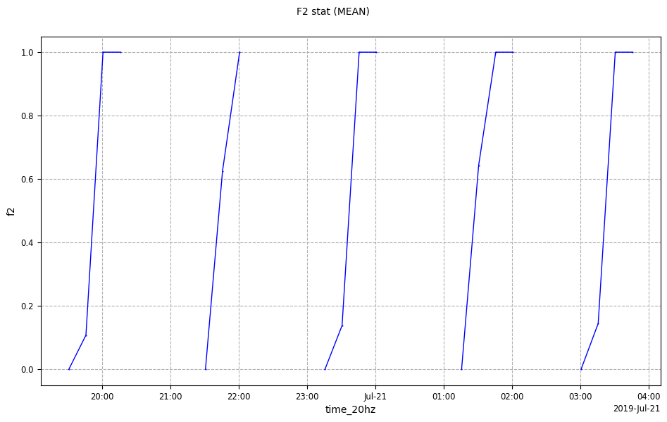
cp2 = CasysPlot(
    data=cd_ncdf, data_name="F2 stat", stat="mean", plot_params=PlotParams(grid=True)
)
cp2.show()