Click here to download this notebook.

How to add custom points to a CasysPlot

CasysPlot objects can be created both from Casys sources (data container like NadirData and SwathData) or from xarray datasets.
Plots can be merged with the method add_plot of CasysPlot objects, allowing to display customi points on top of classic CasysPlot.
This notebook will show some examples.

[1]:

import os

import numpy as np
import xarray as xr

from casys import CasysPlot, NadirData, PlotParams

NadirData.enable_loginfo()

Creating CasysPlot objects from data container

[2]:

# Using the model's computed NadirData object.
ad = NadirData.load(os.environ["DOC_MODEL"])
ad.add_raw_data(name="SIGMA0", field=ad.fields["SIGMA0.ALTI"])
ad.add_geobox_stat(name="SIGMA0 geobox", field=ad.fields["SIGMA0.ALTI"])
ad.compute()

2025-05-14 11:00:53 INFO    Computing diagnostics ['SIGMA0 geobox']
2025-05-14 11:00:53 INFO    Computing done.

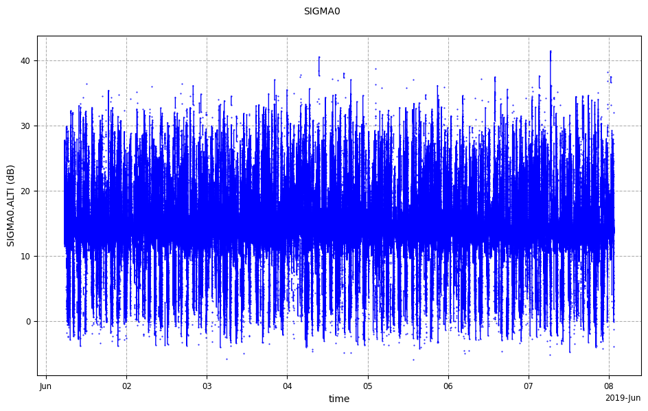
[3]:

plot_casys_raw = CasysPlot(data=ad, data_name="SIGMA0")
plot_casys_raw.show()

[3]:

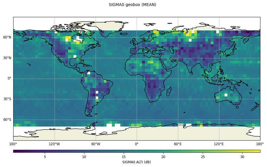
../_images/howto_model_plot_customized_points_5_0.png

[4]:

plot_casys_geobox = CasysPlot(data=ad, data_name="SIGMA0 geobox")
plot_casys_geobox.showi()

../_images/howto_model_plot_customized_points_6_0.png

Creating CasysPlot objects with custom points

Taking a custom set of points:

[5]:

values = np.random.rand(10) * 20 + 15
time = np.arange(
    np.datetime64("2019-06-03"),
    np.datetime64("2019-06-08"),
    np.timedelta64(12, "h").astype(np.timedelta64(1, "ns")),
)
lon = np.random.randint(low=-180, high=180, size=10)
lat = np.random.randint(low=-90, high=90, size=10)

ds_custom_points = xr.Dataset(
    data_vars={
        "CUSTOM_POINTS_VALUES": ("time", values),
        "LONGITUDE": ("time", lon),
        "LATITUDE": ("time", lat),
    },
    coords={"time": time},
)

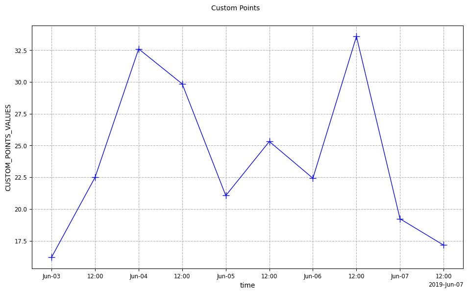
A CasysPlot object can be created using the from_array method.

The dtype parameter indicates the type of plot. Available dtypes and associated usage are detailed here.

For an along time plot of custom data, use dtype="STAT_TIME":

[6]:

plot_custom_time = CasysPlot.from_array(
    name="Custom Points",
    data=ds_custom_points,
    x="time",
    y="CUSTOM_POINTS_VALUES",
    dtype="STAT_TIME",
    plot_params=PlotParams(
        marker_style="+",
        marker_size=10,
    ),
)
plot_custom_time.showi()

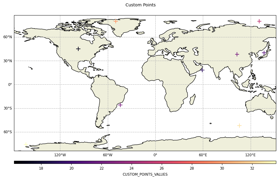
../_images/howto_model_plot_customized_points_12_0.png

For a map plot of the custom data, use dtype="RAW_DATA":

[7]:

plot_custom_map = CasysPlot.from_array(
    name="Custom Points",
    data=ds_custom_points,
    x="LONGITUDE",
    y="LATITUDE",
    z="CUSTOM_POINTS_VALUES",
    time="time",
    dtype="RAW_DATA",
    plot_params=PlotParams(
        marker_style="+",
        marker_size=100,
        color_map="magma",
    ),
)
plot_custom_map.showi()

../_images/howto_model_plot_customized_points_14_0.png

Merging CasysPlot objects

Using the add_plot method of the previously created CasysPlot objects, custom points will be added on the CasysPlot objects created from a data container:

[8]:

plot_casys_raw.add_plot(plot_custom_time)
plot_casys_raw.show()

[8]:

../_images/howto_model_plot_customized_points_17_0.png

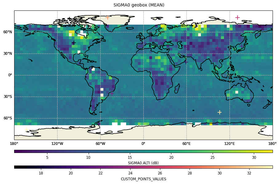
[9]:

plot_casys_geobox.add_plot(plot_custom_map)
plot_casys_geobox.show()

[9]:

../_images/howto_model_plot_customized_points_18_0.png

For more details on merging plots see plots merging documentation.