Click here to download this notebook.

How to add custom data to NadirData

NadirData.data attribute allows to access and enrich the database used by this object [doc].

The following example illustrates how it can be used.

Consider you want to work on a customized selection flag not yet computed in your data source.

import os

import xarray as xr

from casys import NadirData, CasysPlot, DataParams, Field

NadirData.enable_loginfo()

Create and/or load your data

# Using the model's computed NadirData object.
ad = NadirData.load(os.environ["DOC_MODEL"])

ds = ad.data
ds

<xarray.Dataset> Size: 33MB
Dimensions:         (time: 582789)
Coordinates:
  * time            (time) datetime64[ns] 5MB 2019-06-01T05:30:29.807497 ... ...
Data variables:
    LONGITUDE       (time) float64 5MB 17.01 17.14 17.27 ... -123.5 -123.3
    LATITUDE        (time) float64 5MB -66.15 -66.15 -66.15 ... 66.15 66.15
    wind            (time) float64 5MB nan nan nan nan nan ... nan nan nan nan
    SLA             (time) float64 5MB nan nan nan nan nan ... nan nan nan nan
    SIGMA0.ALTI     (time) float64 5MB nan nan nan nan nan ... nan nan nan nan
    EDITING.CUSTOM  (time) int64 5MB 1 1 1 1 1 1 2 1 1 1 ... 1 1 1 1 1 1 1 1 1 1

xarray.Dataset

• Dimensions:
  • time: 582789
• Coordinates: (1)
  • time
    (time)
    datetime64[ns]
    2019-06-01T05:30:29.807497 ... 2...

    standard_name :

    time

    array(['2019-06-01T05:30:29.807497000', '2019-06-01T05:30:30.826208000',
           '2019-06-01T05:30:31.844918000', ..., '2019-06-08T01:28:01.950456000',
           '2019-06-08T01:28:02.969165000', '2019-06-08T01:28:03.987875000'],
          dtype='datetime64[ns]')

• Data variables: (6)
  • LONGITUDE
    (time)
    float64
    17.01 17.14 17.27 ... -123.5 -123.3

    array([  17.006113,   17.135617,   17.265119, ..., -123.587257,
           -123.457709, -123.328159])

  • LATITUDE
    (time)
    float64
    -66.15 -66.15 ... 66.15 66.15

    array([-66.149034, -66.148977, -66.148805, ...,  66.149439,  66.14963 ,
            66.149706])

  • wind
    (time)
    float64
    nan nan nan nan ... nan nan nan nan

    array([nan, nan, nan, ..., nan, nan, nan])

  • SLA
    (time)
    float64
    nan nan nan nan ... nan nan nan nan

    array([nan, nan, nan, ..., nan, nan, nan])

  • SIGMA0.ALTI
    (time)
    float64
    nan nan nan nan ... nan nan nan nan

    array([nan, nan, nan, ..., nan, nan, nan])

  • EDITING.CUSTOM
    (time)
    int64
    1 1 1 1 1 1 2 1 ... 1 1 1 1 1 1 1 1

    array([1, 1, 1, ..., 1, 1, 1])

• Indexes: (1)
  • time
    PandasIndex

    PandasIndex(DatetimeIndex(['2019-06-01 05:30:29.807497', '2019-06-01 05:30:30.826208',
                   '2019-06-01 05:30:31.844918', '2019-06-01 05:30:32.863628',
                   '2019-06-01 05:30:33.882337', '2019-06-01 05:30:34.901048',
                   '2019-06-01 05:30:35.919757', '2019-06-01 05:30:36.938466',
                   '2019-06-01 05:30:37.957177', '2019-06-01 05:30:38.975886',
                   ...
                   '2019-06-08 01:27:54.819487', '2019-06-08 01:27:55.838196',
                   '2019-06-08 01:27:56.856907', '2019-06-08 01:27:57.875616',
                   '2019-06-08 01:27:58.894327', '2019-06-08 01:27:59.913036',
                   '2019-06-08 01:28:00.931746', '2019-06-08 01:28:01.950456',
                   '2019-06-08 01:28:02.969165', '2019-06-08 01:28:03.987875'],
                  dtype='datetime64[ns]', name='time', length=582789, freq=None))

• Attributes: (0)

Compute a new field

You can use any algorithm/custom function here using any external or existing data as parameters.

The only constraint is to be able to make the result fit in your dataset.

# Defining a powerful selection function
def lat_selection(data):
    return xr.where(data["LATITUDE"] > 0, 1, 0)


# Generating the new flag and storing it in our dataset
ds["new_flag"] = lat_selection(ds)

Put everything back into your NadirData

Each new field will be considered as a raw data using the field’s name.

From the outside this operation is similar to ad.add_raw_data(name="new_flag", field=Field("new_flag").

# Setting everything back into our NadirData object
ad.data = ds

Play with your new fields

We can now use the merged fields as any other:

• To compute a statistic

• To create new fields usings CLIPs

# Note: We're using the Python CLIP syntax here (might be confusing but you'll get used to it !).
sla_select = Field(name="SLA_SEL", source="IIF(new_flag:==1, SLA, DV)")
var_wtc_rad_sel = Field(
    name="WTC_SEL",
    source="IIF(new_flag:==1 && FLAG_VAL.ALTI:==0,"
    "WET_TROPOSPHERIC_CORRECTION.RAD, DV)",
)

# These new fields can now be used like any other
ad.add_raw_data(name="SLA selected", field=sla_select)
ad.add_raw_data(name="WTC selected", field=var_wtc_rad_sel)

ad.add_time_stat(name="WTC sel stat", field=var_wtc_rad_sel, freq="15min", stats=["mean"])

ad.compute()

2025-05-14 10:59:36 INFO    Reading ['WET_TROPOSPHERIC_CORRECTION.RAD', 'FLAG_VAL.ALTI']
2025-05-14 10:59:39 INFO    Reading ['WTC_SEL', 'SLA_SEL'] (external source)
2025-05-14 10:59:39 INFO    Computing diagnostics ['WTC sel stat']
2025-05-14 10:59:39 INFO    Computing done.

ad.data

<xarray.Dataset> Size: 47MB
Dimensions:         (time: 582789)
Coordinates:
  * time            (time) datetime64[ns] 5MB 2019-06-01T05:30:29.807497 ... ...
Data variables:
    LONGITUDE       (time) float64 5MB 17.01 17.14 17.27 ... -123.5 -123.3
    LATITUDE        (time) float64 5MB -66.15 -66.15 -66.15 ... 66.15 66.15
    wind            (time) float64 5MB nan nan nan nan nan ... nan nan nan nan
    SLA             (time) float64 5MB nan nan nan nan nan ... nan nan nan nan
    SIGMA0.ALTI     (time) float64 5MB nan nan nan nan nan ... nan nan nan nan
    EDITING.CUSTOM  (time) int64 5MB 1 1 1 1 1 1 2 1 1 1 ... 1 1 1 1 1 1 1 1 1 1
    new_flag        (time) int64 5MB 0 0 0 0 0 0 0 0 0 0 ... 1 1 1 1 1 1 1 1 1 1
    WTC_SEL         (time) float64 5MB nan nan nan nan nan ... nan nan nan nan
    SLA_SEL         (time) float64 5MB nan nan nan nan nan ... nan nan nan nan

xarray.Dataset

• Dimensions:
  • time: 582789
• Coordinates: (1)
  • time
    (time)
    datetime64[ns]
    2019-06-01T05:30:29.807497 ... 2...

    standard_name :

    time

    array(['2019-06-01T05:30:29.807497000', '2019-06-01T05:30:30.826208000',
           '2019-06-01T05:30:31.844918000', ..., '2019-06-08T01:28:01.950456000',
           '2019-06-08T01:28:02.969165000', '2019-06-08T01:28:03.987875000'],
          dtype='datetime64[ns]')

• Data variables: (9)
  • LONGITUDE
    (time)
    float64
    17.01 17.14 17.27 ... -123.5 -123.3

    array([  17.006113,   17.135617,   17.265119, ..., -123.587257,
           -123.457709, -123.328159])

  • LATITUDE
    (time)
    float64
    -66.15 -66.15 ... 66.15 66.15

    array([-66.149034, -66.148977, -66.148805, ...,  66.149439,  66.14963 ,
            66.149706])

  • wind
    (time)
    float64
    nan nan nan nan ... nan nan nan nan

    array([nan, nan, nan, ..., nan, nan, nan])

  • SLA
    (time)
    float64
    nan nan nan nan ... nan nan nan nan

    array([nan, nan, nan, ..., nan, nan, nan])

  • SIGMA0.ALTI
    (time)
    float64
    nan nan nan nan ... nan nan nan nan

    array([nan, nan, nan, ..., nan, nan, nan])

  • EDITING.CUSTOM
    (time)
    int64
    1 1 1 1 1 1 2 1 ... 1 1 1 1 1 1 1 1

    array([1, 1, 1, ..., 1, 1, 1])

  • new_flag
    (time)
    int64
    0 0 0 0 0 0 0 0 ... 1 1 1 1 1 1 1 1

    array([0, 0, 0, ..., 1, 1, 1])

  • WTC_SEL
    (time)
    float64
    nan nan nan nan ... nan nan nan nan

    array([nan, nan, nan, ..., nan, nan, nan])

  • SLA_SEL
    (time)
    float64
    nan nan nan nan ... nan nan nan nan

    array([nan, nan, nan, ..., nan, nan, nan])

• Indexes: (1)
  • time
    PandasIndex

    PandasIndex(DatetimeIndex(['2019-06-01 05:30:29.807497', '2019-06-01 05:30:30.826208',
                   '2019-06-01 05:30:31.844918', '2019-06-01 05:30:32.863628',
                   '2019-06-01 05:30:33.882337', '2019-06-01 05:30:34.901048',
                   '2019-06-01 05:30:35.919757', '2019-06-01 05:30:36.938466',
                   '2019-06-01 05:30:37.957177', '2019-06-01 05:30:38.975886',
                   ...
                   '2019-06-08 01:27:54.819487', '2019-06-08 01:27:55.838196',
                   '2019-06-08 01:27:56.856907', '2019-06-08 01:27:57.875616',
                   '2019-06-08 01:27:58.894327', '2019-06-08 01:27:59.913036',
                   '2019-06-08 01:28:00.931746', '2019-06-08 01:28:01.950456',
                   '2019-06-08 01:28:02.969165', '2019-06-08 01:28:03.987875'],
                  dtype='datetime64[ns]', name='time', length=582789, freq=None))

• Attributes: (0)

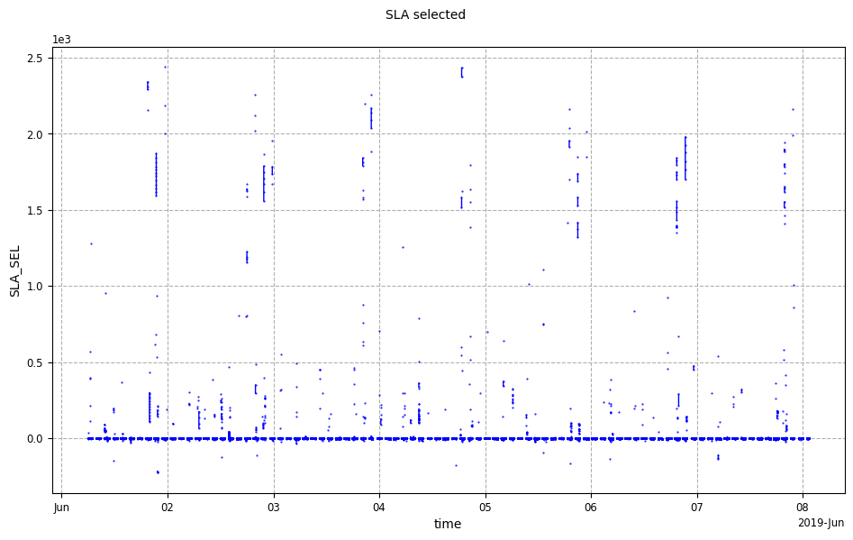
cp_sla = CasysPlot(
    data=ad, data_name="SLA selected", data_params=DataParams(remove_nan=False)
)
cp_sla.show()

cp_sla = CasysPlot(
    data=ad, data_name="SLA selected", data_params=DataParams(remove_nan=True)
)
cp_sla.show()

cp_wtc = CasysPlot(data=ad, data_name="WTC sel stat")
cp_wtc.show()