Click here to download this notebook.

Missing Points

[2]:

import numpy as np

from casys.grids import InGridNetcdfParameters
from casys.readers import CLSTableReader

from casys import CasysPlot, CLSResourcesManager, DateHandler, NadirData

NadirData.enable_loginfo()

Dataset definition

[3]:

# Reader definition
table_name = "TABLE_C_J3_B_GDRD"
start = DateHandler("2019-07-20 19:23:06")
end = DateHandler("2019-07-30 17:21:37")

reader = CLSTableReader(
    name=table_name,
    date_start=start,
    date_end=end,
    time="time",
    longitude="LONGITUDE",
    latitude="LATITUDE",
)

# Data container definition
ad = NadirData(source=reader)

Definition of the diagnostic

The add_missing_points_stat method allows the definition of a missing points diagnostic.

In the following example, we are using a custom grid and grouping function allowing us a more precise differentiation of data according to the bathymetry values.

[4]:

manager = CLSResourcesManager()
grid_path = manager.bathymetry_path("1_12")

params = InGridNetcdfParameters(file_name=grid_path, z_name="Grid_0001")

def bathy_to_groups(x: np.ndarray):
    res = np.empty(x.size)

    res[np.where(x <= -3000)[0]] = 0
    res[np.where((-3000 < x) & (x < 3000))[0]] = 1
    res[np.where((3000 <= x) & (x < 5000))[0]] = 2
    res[np.where(x >= 5000)[0]] = 3

    return res

[5]:

ad.add_missing_points_stat(
    name="Missing points",
    reference_track="J3",
    theoretical_orf="C_J3",
    geobox_stats=True,
    group_names={
        "deep": 0,
        "in-between": 1,
        "high": 2,
        "very high": 3,
        "deep and high": [0, 2],
    },
    group_grid=params,
    group_converter=bathy_to_groups,
    temporal_stats_freq=["pass"],
    section_min_lengths=[64, 128],
)

2025-05-14 10:57:06 WARNING Computed missing points will be using an ORF build with real measurements. Results might be incomplete.

Compute

[6]:

ad.compute()

2025-05-14 10:57:06 INFO    Reading ['time', 'LONGITUDE', 'LATITUDE']
2025-05-14 10:57:09 INFO    Computing diagnostics ['Missing points']
2025-05-14 10:57:09 INFO        Searching missing points.
2025-05-14 10:57:21 INFO    Computing done.

Plot

CasysPlot uses 5 parameters to determine what to plot:

plot: plot’s type (“map”, “temporal”, “geobox”, “section_analyses”)
dtype: “all”, “missing”, “available”
group: “global” (default: data from all groups) or any group defined in the group_names parameter
freq: required for temporal, frequency of the requested statistic
section_min_length: minimal length value of the section analysis to display
sections: optional for section analyses plot

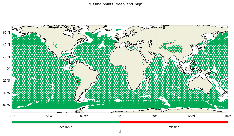
Map plot

Refer to raw data diagnostics documentation for additional information.

Showing all values for the “deep and high” group:

[7]:

plot = CasysPlot(
    data=ad,
    data_name="Missing points",
    plot="map",
    dtype="all",
    group="deep and high",
)

plot.show()

[7]:

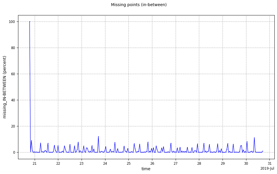
../_images/examples_example_advanced_Missing_Points_15_0.png

Along time diagnostics

Refer to along time diagnostics documentation for additional information.

Showing percentage of missing data for the “in between” group:

[8]:

plot = CasysPlot(
    data=ad,
    data_name="Missing points",
    plot="temporal",
    freq="pass",
    dtype="missing",
    group="in-between",
)

plot.show()

[8]:

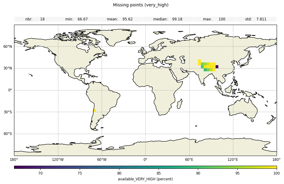
../_images/examples_example_advanced_Missing_Points_18_0.png

Geographical box diagnostics

Refer to geographical box diagnostics documentation for additional information.

Showing available data percentage as geographical boxes for the “high” group:

[9]:

plot = CasysPlot(
    data=ad,
    data_name="Missing points",
    plot="geobox",
    dtype="available",
    group="very high",
)

plot.add_stat_bar()
plot.show()

[9]:

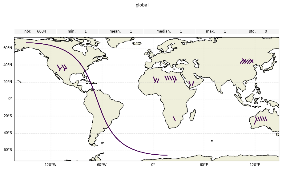
../_images/examples_example_advanced_Missing_Points_21_0.png

Section Analysis diagnostics

Refer to section analysis diagnostics documentation for additional information.

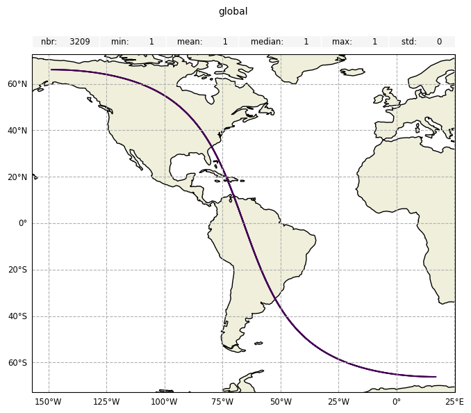
Showing all sections for missing points for the “global” group (default) and section_min_length=64:

[10]:

plot = CasysPlot(
    data=ad,
    data_name="Missing points",
    plot="section_analyses",
    section_min_length=64,
)

plot.add_stat_bar()
plot.show()

[10]:

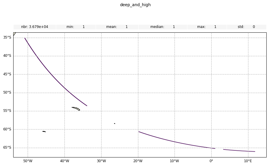
../_images/examples_example_advanced_Missing_Points_24_0.png

Showing all sections for missing points for the “deep and high” group and section_min_length=64:

[11]:

plot = CasysPlot(
    data=ad,
    data_name="Missing points",
    plot="section_analyses",
    group="deep and high",
    section_min_length=64,
)

plot.add_stat_bar()
plot.show()

[11]:

../_images/examples_example_advanced_Missing_Points_26_0.png

Showing all sections for missing points for the “global” group and section_min_length=128:

[12]:

plot = CasysPlot(
    data=ad,
    data_name="Missing points",
    plot="section_analyses",
    section_min_length=128,
)

plot.add_stat_bar()
plot.show()

[12]:

../_images/examples_example_advanced_Missing_Points_28_0.png

Selecting only the sections 2 and 3 for “global” group and section_min_length=64:

[13]:

plot = CasysPlot(
    data=ad,
    data_name="Missing points",
    plot="section_analyses",
    section_min_length=64,
    sections=[2, 3],
)

plot.add_stat_bar()
plot.show()

[13]:

../_images/examples_example_advanced_Missing_Points_30_0.png

To learn more about missing points definition, please visit this documentation page.