Raw along track data diagnostics

Raw data are added using the add_raw_data() method. Fields data will be extracted alongside their time, longitude and latitude coordinates.

Warning

When using a SwathData data container, the amount of data is important, so Raw diagnostics should only be used to visualize short time periods.

Add a raw data diagnostic (used for along track plotting).

Raw data and plots can be accessed or created using special keywords:

 * plot="time" (default): along time representation.
 * plot="map": Cartographic representation.
 * plot="3d": 3d scatter representation.

Parameters
----------
name
    Name of the diagnostic.
field
    Field for which to get raw data.

Raises
------
AltiDataError
    If a diagnostic already exists with the provided name.

These data can then be accessed through the data property to explore their numerical values (additional information may be found here.)

Or plotted:

as an along time plot using the option: plot=”time” when initializing the CasysPlot object (default value).

as a map plot: plot=”map” when initializing the CasysPlot object.

Diagnostic setting

In the following example, we are setting a raw diagnostic:

for an existing field SIGMA0.ALTI in the NadirData.

sig0 = ad.fields["SIGMA0.ALTI"]

ad.add_raw_data(name="Sigma 0", field=sig0)

ad.compute()

for an existing field swh_karin in the SwathData.

swh_karin = sd.fields["swh_karin"]

sd.add_raw_data(name="SWH Karin", field=swh_karin)

sd.compute()

Diagnostic plotting

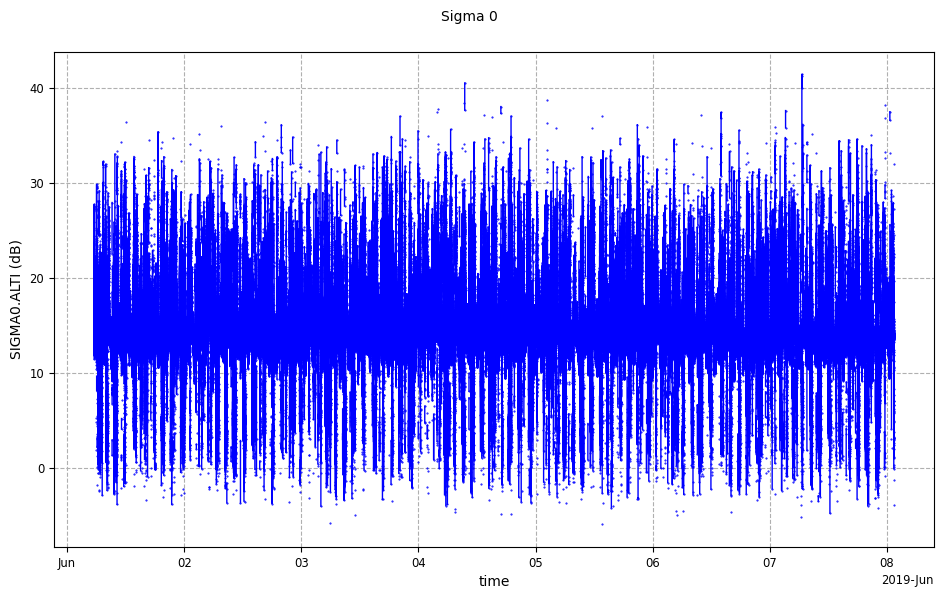
CasysPlot requires a plot parameter to be given in order to know which plotting to use.

Along time plot

Along time plots require the plot parameter to have the “time” value.

This is the default value and can omitted.

from casys import CasysPlot

plot = CasysPlot(data=ad, data_name="Sigma 0", plot="time")

plot.show()

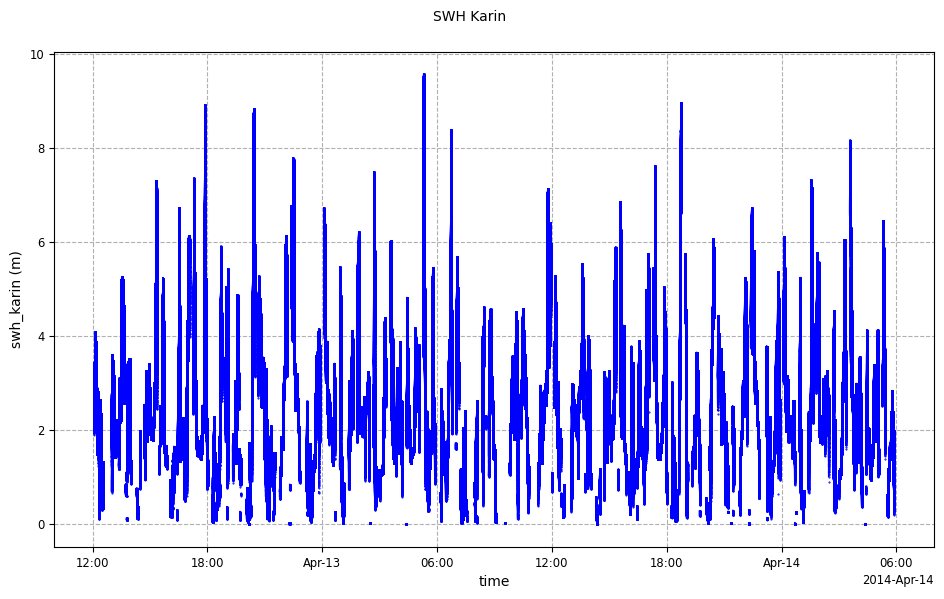
For SwathData data container, the time period to visualize might be limited in order to reduce the quantity of points to display.

from casys import DataParams, DateHandler

time_limits = (
    DateHandler("2014-04-12 15:00:00"),
    DateHandler("2014-04-12 15:01:00"),
)

plot = CasysPlot(data=sd,
    data_name="SWH Karin",
    plot="time",
    data_params=DataParams(
        time_limits=time_limits,
    ),
)

plot.show()

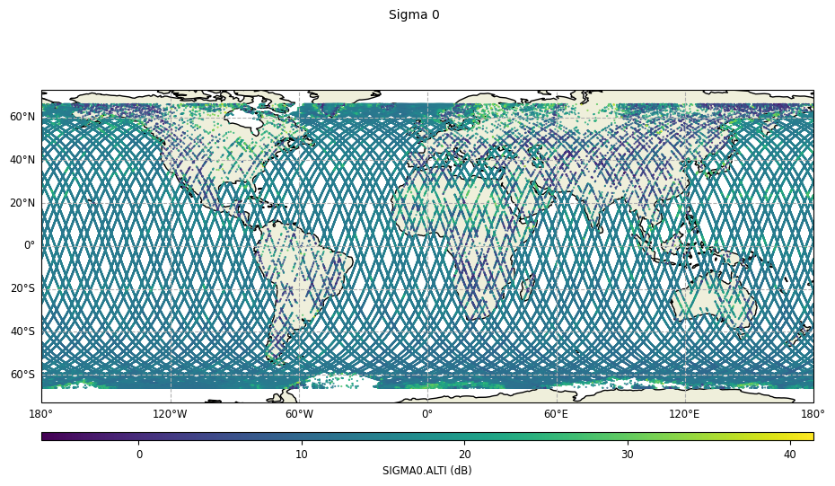
Map plot

Map plots require the plot parameter to have the “map” value.

plot = CasysPlot(data=ad, data_name="Sigma 0", plot="map")

plot.show()

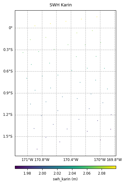
You might want to use the points_min_radius parameter when visualizing swath data.

time_limits = (
    DateHandler("2014-04-12 15:00:00"),
    DateHandler("2014-04-12 15:00:30"),
)

plot = CasysPlot(
    data=sd,
    data_name="SWH Karin",
    plot="map",
    data_params=DataParams(
        time_limits=time_limits,
        points_min_radius=0.2,
    ),
)

plot.show()

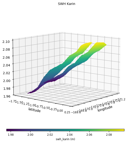
3D plot

3D plots require the plot parameter to have the “3d” value.

NadirData containers will plot data with as a scatter:

plot = CasysPlot(data=ad, data_name="Sigma 0", plot="3D")

plot.show()

SwathData data will be plotted as surfaces

The two swaths of the data can be split using plot="3d:n_pix", with n_pix the index of the splitting pixel.

In the same way as 2D plot, you might want to use the points_min_radius parameter when visualizing swath data.

time_limits = (
    DateHandler("2014-04-12 15:00:00"),
    DateHandler("2014-04-12 15:00:30"),
)

plot = CasysPlot(
    data=sd,
    data_name="SWH Karin",
    plot="3D:35",
    data_params=DataParams(
        time_limits=time_limits,
        points_min_radius=0.1,
    ),
)

plot.show()