Histogram diagnostics

Histograms diagnostics are added using the add_histogram() method.

Provided field distribution will be computed according to the res_x parameter.

Add a histogram diagnostic for the provided field computing its
values' distribution according to the res_x parameter.

Parameters
----------
name
    Name of the diagnostic.
x
    Field used for the x-axis.
res_x
    Min, max and width for the x-axis, 'auto' (Default: 'auto').
    'auto' will use the 2.5 percentile of values as min, the 97.5 percentile
    as maximum and make 40 groups in between.

This kind of diagnostic is plotted as a bar or curve plot and can be normalized at plotting time.

Diagnostic setting

In the following example we are setting an histogram diagnostic for a user defined SLA field for values between -6 and 0 with a step of 0.05.

from casys import Field

sla = Field(
    name="SLA",
    source="ORBIT.ALTI - RANGE.ALTI - MEAN_SEA_SURFACE.MODEL.CNESCLS15",
    unit="m",
)

ad.add_histogram(
    name="Histo sla",
    x=sla,
    res_x=(-6, 0, 0.05),
)

ad.compute()

Diagnostic plotting

Histogram diagnostics are plotted as bar plots by default. They can be plotted as curve as well by providing a PlotParams with its bars parameter set to False.

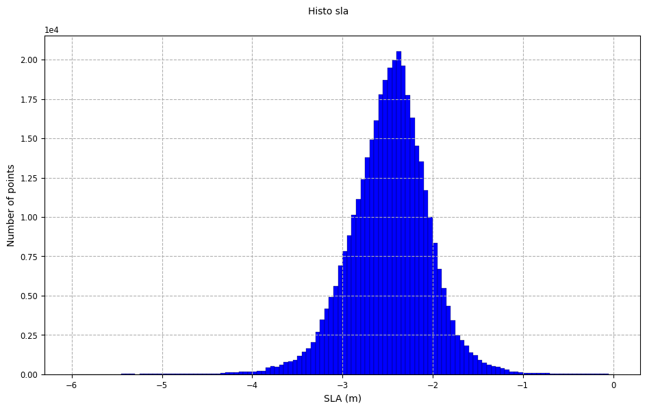
Histograms values can be normalized as a percentage of the total number of values using a DataParams with its normalize parameter set to True.

Bar plot

from casys import CasysPlot

plot = CasysPlot(data=ad, data_name="Histo sla")

plot.show()

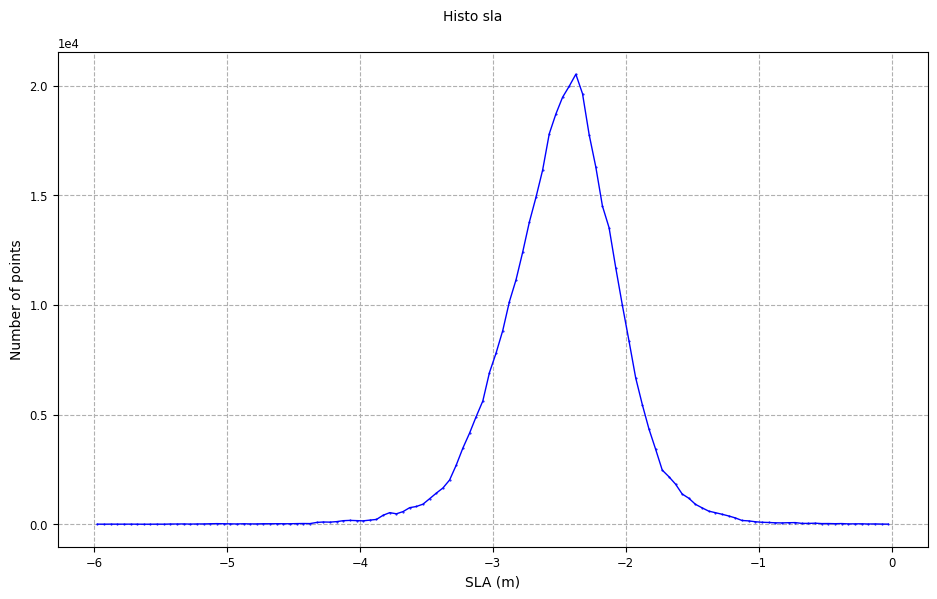
Curve plot

from casys import PlotParams

plot = CasysPlot(
    data=ad,
    data_name="Histo sla",
    plot_params=PlotParams(bars=False),
)

plot.show()

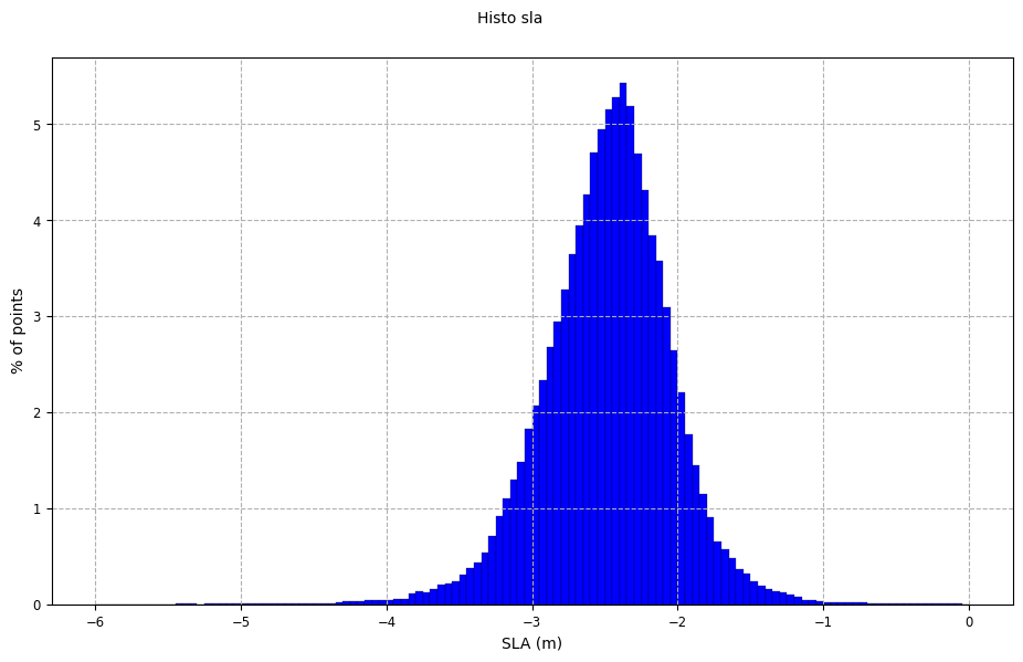
Normalized plot

from casys import DataParams

plot = CasysPlot(
    data=ad,
    data_name="Histo sla",
    data_params=DataParams(normalize=True),
)

plot.show()