Crossovers diagnostics - Swath

Crossovers diagnostics are added using the add_crossover_stat() method of the SwathData() container.

It allows the computation of the difference between the ascending and descending arcs at crossover locations for the provided field.

For SwathData, a crossover is defined by several points, forming an area called a crossover diamond.

For each crossover, the diagnostic computes:

• the difference between the field values of the two arcs

• the difference between the time values of the two arcs

In addition, diagnostics are computed on the difference of field values of the two arcs:

• geographical box diagnostics using the parameters:

  • stats or geobox_stats

  • res_lon

  • res_lat

• [optional] along time diagnostics using the parameters:

  • stats or temporal_stats

  • temporal_stats_freq

  • temporal_freq_kwargs: dictionary of additional parameters to pass to the pandas.date_range underlying function

Note

The stats parameter is used in instance where the statistics to compute for temporal and geobox sub-diagnostics are the same.

If geobox_stats and/or temporal_stats are also defined, their value will be used in priority.

Using diamond_reduction, diamond_relocation, cartesian_plane and crossover_table parameters, add_crossover_stat() allows to customize the search for crossovers and reformat the results.

Several other parameters will affect the computation of the crossovers locations, as:

• pass_multi_intersect: whether to look for multiple intersections between a set of two passes or not.

• cartesian_plane: flag determining the plane used for crossovers computation.

• crossover_table: the table of possible combinations of crossovers between the two passes.

Add the computation of the difference between the ascending and
descending arc values in the crossovers diamonds or at crossovers
equivalent Nadir points (see diamond_reduction parameter for a
statistical reduction of the diamond data). Temporal statistics (by
cycle or day) can be added to the computation.

Values and time delta are computed at each point and requested statistics for
each geographical box. These data are accessible using the requested statistics
name or 'crossover' and 'value' keywords for the time delta and the values at
each crossover point.

Crossovers data and plots can be accessed or created using special keywords:

* delta parameter: cartographic representation of the difference
  between the two arcs

    * delta="field": difference of the field values
    * delta="time": difference of the time values

* stat parameter: geographical box or temporal statistic representation.

    * stat="...": requested statistic

* freq parameter: temporal statistic representation.

    * freq="...": frequency of the requested statistic

Parameters
----------
name
    Name of the diagnostic.
field
    Field for which to compute the statistic.
data
    External data (NadirData) to compute crossovers with.
    This option is used to compute multi-missions crossovers.
max_time_difference
    Maximum delta of time between the two arcs as a string with its unit.
    Any string accepted by pandas.Timedelta is valid.
    i.e. '10 days', '6 hours', '1 min', ...
stats
    List of statistics to compute (count, max, mean, median, min, std, var,
    mad) for temporal and geobox statistics.
res_lon
    Minimum, maximum and box size over the longitude (Default:  -180, 180, 4).
res_lat
    Minimum, maximum and box size over the latitude (Default:  -90, 90, 4).
box_selection
    Field used as selection for computation of the ``count`` statistic.
    Box in which the box_selection field does not contain any data will be set
    to NaN instead of 0.
geobox_stats
    Statistics included in the geobox diagnostic.
temporal_stats_freq
    List of temporal statistics frequencies to compute.
temporal_stats
    Statistics included in the temporal diagnostic.
temporal_freq_kwargs
    Additional parameters to pass to pandas.date_range underlying function.
pass_multi_intersect
    Whether to look for multiple intersections between a set of 2 passes or not.
cartesian_plane
    Flag determining the plane used for crossovers computation.
    If True, the crossover is calculated in the cartesian plane.
    If False, the crossover is calculated in the spherical plane.
    Defaults to True.
crossover_table
    The table of possible combinations of crossovers between the two passes.
    If this table is not defined, all crossovers between odd and even passes
    will be calculated.
diamond_relocation
    Flag determining data relocation to nadir crossover coordinates for
    the statistics computation.
    If True, data relocation is performed. Default value is False.
diamond_reduction
    Statistic type used to reduce the data on the crossover diamond.
    Reduction is disabled with the "none" value.
    (Default value is "mean")

Raises
------
AltiDataError
    If a data already exists with the provided name.

Like for NadirData, this kind of diagnostic can generate up to 3 kinds of plots:

• raw data diagnostics map plots for time and field differences

• along time diagnostics plots

• geographical box diagnostics plots

Mono-mission Swath/Swath crossovers

Diagnostic setting

In the following example we are setting a crossovers diagnostic for the user defined field swh computing a geographical box diagnostics with default parameters and an along time diagnostics at day and ‘one hour’ frequencies.

First possibility, the mean and count statistics (defined with stats) are computed for both sub diagnostics.

Second possibility, the mean and count statistics (defined with geobox_stats) are computed for the geobox sub diagnostic, and the std and count statistics (defined with temporal_stats) for the temporal sub diagnostic.

Like for simple temporal diagnostic, the temporal_freq_kwargs parameter allows to pass additional parameters to the pandas.date_range underlying function, for custom frequency values.

As mentioned previously, the area formed by the ascending and descending arcs crossover is called a crossover diamond.

Concerning the data of crossover diamonds, the statistics computation can be performed on the original diamond data (with diamond geometry) or on the data relocated to the corresponding nadir crossover.

To relocate the diamond data, the flag parameter diamond_relocation must be set to True.

The diamond_reduction parameter allows to reduce the data to the corresponding nadir coordinates, by specifying the statistical reduction method.

The diamond_reduction default value is mean.

The remaining available parameters are:

• cartesian_plane: flag to determine if crossovers are computed in the cartesian place,

• crossover_table: table of possible combinations of crosssovers between available passes.

from casys import Field

var_swh = Field(
    name="swh_karin",
    unit="m",
)

sd.add_crossover_stat(
    name="Crossover SWH 1",
    field=var_swh,
    max_time_difference="5 days",
    stats=["mean", "count"],
    temporal_stats_freq=["day", "1h"],
    diamond_relocation=False,
    diamond_reduction="mean",
)

sd.add_crossover_stat(
    name="Crossover SWH 2",
    field=var_swh,
    max_time_difference="5 days",
    geobox_stats=["mean", "count"],
    temporal_stats=["std", "count"],
    temporal_stats_freq=["day", "1h"],
    diamond_relocation=True,
    diamond_reduction="mean",
)

sd.add_crossover_stat(
    name="Crossover SWH 3",
    field=var_swh,
    max_time_difference="5 days",
    stats=["mean", "count"],
    temporal_stats_freq=["20min", "1h"],
    temporal_freq_kwargs={"normalize": True},
    diamond_relocation=False,
    diamond_reduction="none",
)

sd.compute()

Diagnostic plotting

Like for NadirData case, CasysPlot uses 3 parameters to determine what to plot:

• delta: plots time or field differences at crossovers

  • delta = “field”

  • delta = “time”

• stat: plots geographical box diagnostics

• stat + freq: plots along time diagnostics

Field and time differences at crossovers

Crossovers field and time diagnostics are plotted as raw data diagnostics map plots.

Note

Time differences might contain more points than field differences if the field is not defined at some crossover points.

Time differences.

from casys import CasysPlot

plot = CasysPlot(data=sd, data_name="Crossover SWH 1", delta="time")

plot.show()

Field differences.

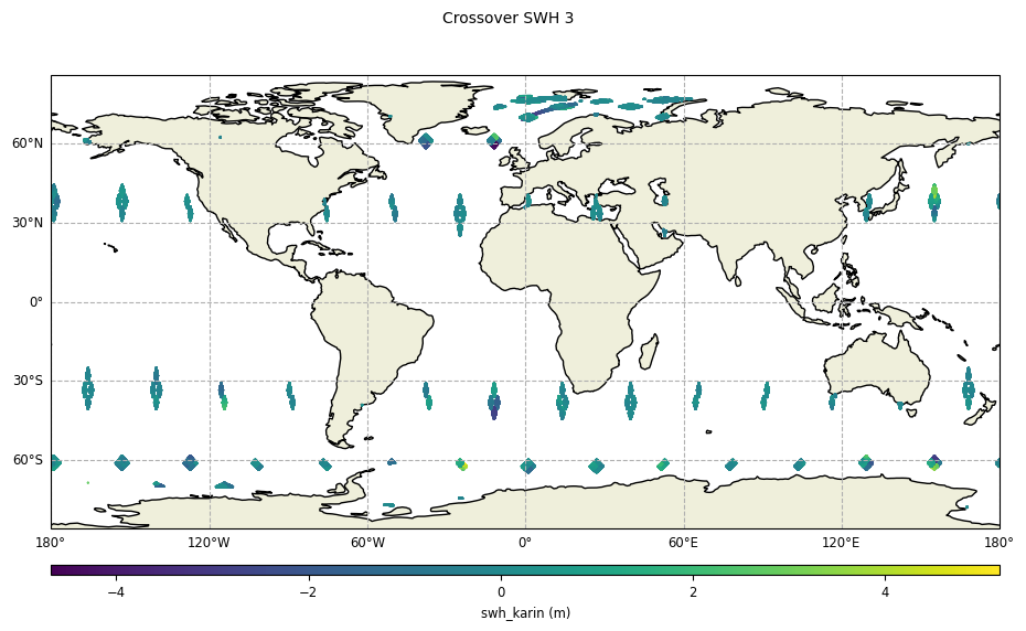
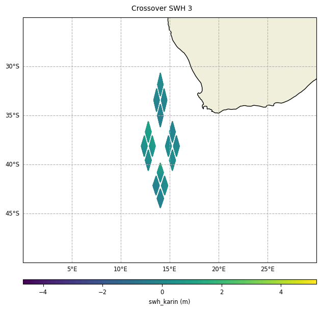
• Without reduction of crossover diamonds, diamond_reduction="none":

plot = CasysPlot(data=sd, data_name="Crossover SWH 3", delta="field")

plot.show()

All the crossover diamond points are kept:

from casys import PlotParams

plot = CasysPlot(
    data=sd,
    data_name="Crossover SWH 3",
    delta="field",
    plot_params=PlotParams(x_limits=(0, 30), y_limits=(-50, -25),),
)

plot.show()

• With reduction of crossover diamonds, diamond_reduction="mean":

plot = CasysPlot(data=sd, data_name="Crossover SWH 1", delta="field")

plot.show()

Crossover diamonds are reduced to the corresponding nadir coordinates:

plot = CasysPlot(
    data=sd,
    data_name="Crossover SWH 1",
    delta="field",
    plot_params=PlotParams(x_limits=(0, 30), y_limits=(-50, -25), marker_size=10),
)

plot.show()

Along time diagnostics

Refer to along time diagnostics documentation for additional information.

plot = CasysPlot(data=sd, data_name="Crossover SWH 1", freq="1h", stat="mean")

plot.show()

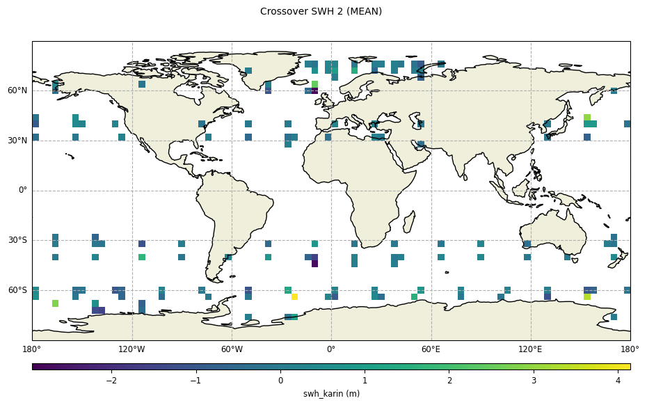
Geographical box diagnostics

Refer to geographical box diagnostics documentation for additional information.

The data displayed on these plot varies with the diamond_relocation flag parameter value.

• for diamond_relocation=False

plot = CasysPlot(data=sd, data_name="Crossover SWH 1", stat="mean")

plot.show()

• for diamond_relocation=True

plot = CasysPlot(data=sd, data_name="Crossover SWH 2", stat="mean")

plot.show()

Multi-missions Swath/Nadir crossovers

Crossovers can also be computed between two different sets of data.

Using the data parameter of the add_crossover_stat() method allows to calculate crossovers with a NadirData.

Diagnostic setting

Note

The Field’s source_aux parameter allows to configure a field having a different source in each NadirData

The following example compute crossovers between the swath type data and classic nadir data (ad):

var_swh = Field(name="swh_karin", source_aux="SWH.ALTI")

sd.add_crossover_stat(
    name="Crossover Swath Nadir",
    field=var_swh,
    data=ad,
    max_time_difference="11 days",
    temporal_stats_freq=["day", "1h"],
    stats=["std", "mean"],
    diamond_reduction="mean",
)

sd.compute()

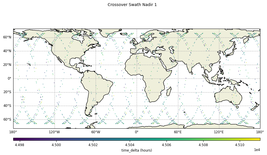
Diagnostic plotting

Swath/Nadir crossovers plotting is done in the exact same manner as Swath/Swath crossovers.

The computation of the difference at crossovers is done by removing the SwathData field data to the NadirData field data.

Time differences.

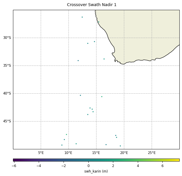
plot = CasysPlot(data=sd, data_name="Crossover Swath Nadir 1", delta="time")

plot.show()

Field differences.

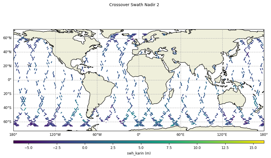
• Without reduction of crossover diamonds, diamond_reduction="none":

plot = CasysPlot(data=sd, data_name="Crossover Swath Nadir 2", delta="field")

plot.show()

All the crossover points are kept:

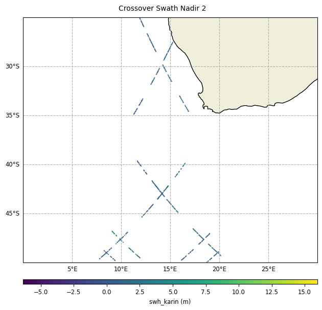
plot = CasysPlot(
    data=sd,
    data_name="Crossover Swath Nadir 2",
    delta="field",
    plot_params=PlotParams(x_limits=(0, 30), y_limits=(-50, -25)),
)

plot.show()

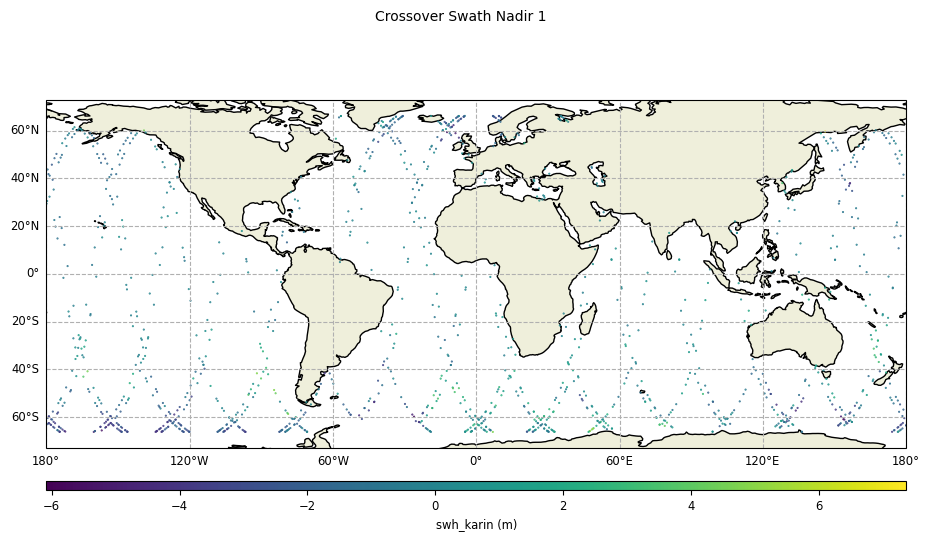
• With reduction of crossover diamonds, diamond_reduction="mean":

plot = CasysPlot(data=sd, data_name="Crossover Swath Nadir 1", delta="field")

plot.show()

Crossover points are reduced to the corresponding nadir coordinates:

plot = CasysPlot(
    data=sd,
    data_name="Crossover Swath Nadir 1",
    delta="field",
    plot_params=PlotParams(x_limits=(0, 30), y_limits=(-50, -25), marker_size=10),
)

plot.show()