Spectral analysis

This diagnostic parameters and results varies depending on the data container used: NadirData() or SwathData().

For both containers, spectral analysis diagnostics are added using the add_spectral_analysis metonhod of the used data container.

It allows the computation of the spectral analysis for the provided field, by completing the following steps:

Selecting valid data segments
Computing the spectral curves

According to the provided parameters, for the segments selection:

segment_length: length of a segment. Needs to be provided.
holes_max_length: maximum length of a hole (Default: 1% of the ``segment_length`` value).
global_resampling: resampling flag (Default: False).
delta_t: time gap between two measurements.
noise_amplitude: noise amplitude in data (Default: half of the data standard deviation).
insulation_level: minimum valid values percentage on both sides of the hole (Default: 0.75).
last_segment_overlapping: percentage of overlap for second-to-last segment (Default: 0)
max_time_dispersion: maximum allowed percentage of dispersion for delta_t (Default: 5).
max_resampling: maximum resampled data percentage (Default: 0.25).
segments_nb_delta_t: number of segments used to compute the average time gap between two measurements, during the segments extraction process (Default: 1).
segments_nb_delta_x: number of segments used to compute the average distance between two measurements, during the segments extraction process (Default: 1).

The last two parameters, segments_nb_delta_t and segments_nb_delta_x, are used for non constant step cases.

The following table indicates the number of points corresponding to a 1000 km segment length depending on the mission characteristics:

${\Delta}t_1$ stands for the low resolution (or normal resolution) time delta, in seconds.
${\Delta}t_2$ stands for the high resolution time delta, in seconds.
${\nu}_1$ and ${\nu}_2$ are the frequency in Hz corresponding to ${\Delta}t_1$ and ${\Delta}t_2$ .

The number of points are obtained for a given segment length, using the following formula:

$nb_{pts} = \frac{length_{segment}}{spd_{ground} \times \Delta_t}$

Mission	Ground speed (km/s)	${\Delta}t_1$ (s)	${\nu}_1$ (Hz)	pts nb @ ${\nu}_1$	${\Delta}t_2$ (s)	${\nu}_2$ (Hz)	pts nb @ ${\nu}_2$
Topex/Poseidon (TP)	5.77	1.07858	1	161
Jason1 (J1)	5.77	1.02	1	170	0.051	20	3398
Jason2 and Jason3 (J2/J3)	5.77	1.01941747572816	1	170	0.0509708737864078	20	3400
Sentinel-6 (S6A)	6.7	1	1	173	0.05	20	3466
Sentinel-3 (S3A/S3B)	6.7	1	1	149	0.0476190476190476	20	3134
SARAL/AltiKa (AL)	6.73	1.04	1	142	0.026	40	5715
Cryosat-2 (C2)	6.77	0.9434	1	157	0.04717	20	3131
HY-2 (H2/H2B/H2C)	6.337	1.024	1	154	0.0512	20	3082
CFOSAT (CFO)	7.03	10.857			0.21714	5	655

For more detailed on each parameters, see the add_spectral_analysis() documentation.

And for the spectral analysis results:

spectral_conf: dictionary defining the parameters used to perform the spectral analysis,

res_segments: flag to indicate whether or not to keep the segments data in the results (Default:False),

res_individual_psd: flag to indicate whether or not to keep the individual power spectrum on each segments, before averaging (Default:False).

The spectral_conf parameter has the following format:

spectral_conf = {
    "sp_analysis_name_1": {
        "spectral_type": "periodogram", "param_11": param_11_value, "param_12": param_12_value, ..
    },
    "sp_analysis_name_2": {
        "spectral_type": "periodogram", "param_21": param_21_value, "param_22": param_22_value, ...
    },
    ...
    "sp_analysis_name_n": {
        "spectral_type": "welch", "param_n1": param_n1_value, "param_n2": param_n2_value, ...
    },
}

The spectral_analysis_name_n is the custom name of the nth spectral analysis configuration for the psd computation.

For each sub configuration in the spectral_conf parameter, the spectral_type parameter is mandatory.
The two available values for spectral_type are periodogram and welch.
The computation for those two spectral types are using the corresponding scipy functions:

For all the other parameters, default values are set if not provided in the spectral_conf parameter:

periodogram:

{'detrend': 'linear',
 'nfft': None,
 'return_onesided': True,
 'scaling': 'density',
 'window': ('tukey', 0.05)}

welch:

{'average': 'mean',
 'detrend': 'linear',
 'nfft': None,
 'noverlap': 0,
 'nperseg': None,
 'return_onesided': True,
 'scaling': 'density',
 'window': ('tukey', 0.05)}

For the window parameter, if the value is a string or tuple, it is passed to the scipy.signal.get_window function to generate the window values:

a character chain: name of the window to use ("hann")
a tuple: name of the window to use and additional parameters (("tukey", 0.2))

See get_window for a list of windows and required parameters.

If window is array_like it will be used directly as the window and its length must be equal to segment_length value.

For NadirData, there is only one pixel along the pass.
For SwathData, several pixels can be selected to compute the spectral analysis.
The difference results in several additional parameters.

First one is the pixels parameter, allowing to select the pixel values to perform the spectral analysis on.

This parameter is a list or tuple of:

single integer/float values indicating a single pixel value: pix

lists/tuples of two integer values indicating a range of pixel values: [pix_min, pix_max]

It is also possible to provide a single integer value for a single pixel in the spectral analysis.

Let’s see the following pixels format examples:

# Single pixel
pixels = 20
pixels = (20)
pixels = [20]

# Several pixels
pixels = [55, 60]
pixels = (55, 60)

# Single pixels range
pixels = [[55, 60]]
pixels = [(55, 60)]
pixels = ([55, 60])
pixels = ((55, 60))

# Several pixels and pixels ranges
pixels = [20, [55, 60], 49, [15, 18]]
pixels = [20, (55, 60), 49, (15, 18)]
pixels = (20, [55, 60], 49, [15, 18])
pixels = (20, (55, 60), 49, (15, 18))

In each category, all the examples are equivalent and the spectral analysis would be performed for:

single pixel: the pixel value 20,

several pixels: pixel values 55 and 60,

single pixels range: pixel values between 55 and 60,

several pixels and pixels range: pixel values equal to 20 and 49

and pixels values between 55 and 60 and between 15 and 18.

Two other parameters, pixels_selection and pixels_reduction, allows to choose the final results content: the potential results reduction and the method of reduction.

The pixels_reduction parameter define the method of reduction, like mean or std for example.

For the pixels_selection parameter, the different possibilities available are:

none: spectral analyses are kept for each pixel value
all: reduction of all spectral analyses to a single spectral analysis
range: reduction of spectral analyses contained in ranges (pix_min, pix_max) of the pixels parameter

The default pixels_selection value is range.

For the previous pixels example, the results would be depending on the pixels_selection value:

pixels pixels_selection	“none”	“all”	“range”
20	1 result for 20	1 result for 20	1 result for 20
[55, 60]	2 results: 55, 60	1 result reduced from: 55, 60	2 results: 55, 60 (no range here)
[[55, 60]]	6 results: 55, 56, 57, 58, 59, 60	1 result reduced from: 55, 56, 57, 58, 59, 60	1 result reduced from: 55, 56, 57, 58, 59, 60
[20, (55, 60), 49, (15, 18)]	11 results: 20, 55, 56, 57, 58, 59, 60, 49, 15, 16, 17, 18	1 result reduced from: 20, 55, 56, 57, 58, 59, 60, 49, 15, 16, 17, 18	4 results: - 1 for 20 - 1 reduced from: 55, 56, 57, 58, 59, 60 - 1 for 49 - reduced from: 15, 16, 17, 18

When performing a reduction on a set of spectral analysis results, only the segments data of the first spectral analysis results is kept (if res_segments=True).

For more detailed on each parameters, see the add_spectral_analysis() documentation.

Nadir Data

Spectral analysis diagnostics are added using the add_spectral_analysis() method.

Add the computation of a spectral analysis diagnostic.

Spectral analysis data and plots can be accessed or created
using special keywords:

 * plot="psd" (default): Power spectral density along the wave number,
 * plot="segments": Cartographic representation of the selected segments.

In the plot="psd" case, a "spectral_name" parameter must be provided to
specify the required spectral analysis. If not, data of the first spectral
analysis will be returned.

The ``segments_reduction`` parameter also needs to be provided if more than
one reduction was requested or if computed using dask:

 * segments_reduction="mean"
 * segments_reduction="median"

Additional plotting options are available to the "psd" plot type:

 * individual: setting it to ``True`` (Default: ``False``) display the set of
   psd on each segments instead of the average psd,
 * n_bins_psd: integer determining the number of bins along the psd values
   axis for the individual=True case (Default: 100),
 * second_axis: flag allowing the display of the second x-axis, for the
   segment length values equivalent to the wave number.

Parameters
----------
name
    Name of the diagnostic.
field
    Field on which to compute the analysis.
segment_length
    Length of a segment (section) in number of points.
    It should be something like a few hundred points. (Example: 500 units)
holes_max_length
    Maximum length of a hole. It should be something like a few points.
    (Example: 5, Default: 1% of the segment_length parameter value)
global_resampling
    Resampling Flag (Default: False).
    True - If one section requires to be resampled => resample all sections.
    False - Resample only  sections requiring a resampling.
delta_t
    Time gap between two measurements.
noise_amplitude
    Noise amplitude in data.
    Default to half of the data standard deviation.
insulation_level
    Minimum valid values percentage on both sides of the hole (Default: 0.75).
    Left and right sides are equal to hole length.
last_segment_overlapping
    Percentage of overlap for second-to-last segment (Default: 0.5).
    When the section is divided in equal segments, the last segment might be
    too short, so it will take some part of data (amount depending on this
    parameter) from the previous segment.
max_time_dispersion
    Maximum allowed percentage of dispersion for delta_t (Default: 5).
    If delta_t dispersion exceed this threshold, a warning will be displayed.
max_resampling
    Maximum resampled data percentage (Default: 0.25).
    A warning will be displayed if this threshold is exceeded.
    The resampling of a large amount of data can have a great impact on the
    final result.
segments_nb_delta_t
    Number of segments used to compute the average time gap between two
    measurements, during the segments extraction process (Default: 1).
segments_nb_delta_x
    Number of segments used to compute the average distance between two
    measurements, during the segments extraction process (Default: 1).
spectral_conf
    Dictionary of the spectral parameters to use for the spectral curve types.
    Each key represents a spectral analysis name is associated with a dictionary
    containing the parameters. This dictionary must contain at least the
    "spectral_type" key and value. (Default: dictionary containing
    the default "periodogram" parameters:
    {"periodogram": {"spectral_type": "periodogram",
    "window": "hann", "detrend": "linear",  ...}}).
segments_reduction
    List of statistic types used to reduce the spectral data across segments
    (Default: mean).
res_segments
    Flag indicating whether to save the segments data
    in the spectral analysis result (Default: False).
    True - Saving segments data.
    False - Not saving segments data.
res_individual_psd
    Flag indicating whether to save the individual
    power spectrum data on each segments
    in the spectral analysis result (Default: False).
    True - Saving the individual psd data.
    False - Not saving the individual psd data.

This kind of diagnostic can generate 2 kind of plots:

raw data diagnostics map plots for segments selected for the spectral analysis

spectral power density curves plots

Diagnostic setting

In the following example we are setting a spectral analysis diagnostic for the user defined field sla.

from casys import Field

var_sla = Field(
    name="SLA",
    source="ORBIT.ALTI - RANGE.ALTI - MEAN_SEA_SURFACE.MODEL.CNESCLS15",
    unit="m",
)

ad.add_spectral_analysis(
    name="Spectral SLA 1",
    field=var_sla,
    segment_length=1024,
    holes_max_length=64,
    spectral_conf={
        "Periodogram, Tukey (alpha=0.2)": {
            "spectral_type": "periodogram",
            "detrend": "linear",
            "window": ("tukey", 0.2),
        },
        "Periodogram, Blackmanharris": {
            "spectral_type": "periodogram",
            "window": "blackmanharris",
        },
        "Welch, Tukey (alpha=0.2)": {
            "spectral_type": "welch",
            "detrend": "linear",
            "window": ("tukey", 0.2),
        },
    },
    res_segments=True,
    res_individual_psd=True,
)

ad.add_spectral_analysis(
    name="Spectral SLA 2",
    field=var_sla,
    segment_length=2048,
    holes_max_length=64,
    res_segments=True,
    spectral_conf={
        "Periodogram, Tukey (alpha=0.2)": {
            "spectral_type": "periodogram",
            "detrend": "linear",
            "window": ("tukey", 0.2),
        },
    },
)

ad.compute()

Diagnostic plotting

CasysPlot uses the plot parameter to determine what to plot:

plot: plots segments map or spectral power density curves

plot = “segments”

plot = “psd”

For plot = “psd”, an additional parameter is available: spectral_name.

It indicates the spectral analysis result to display. The value must be one of the sub configuration name in the spectral_conf parameter provided at the diagnostic creation.

Segments plotting

Segments diagnostics are plotted as raw data diagnostics map plots.

segment_length = 1024

from casys import CasysPlot, DataParams

plot = CasysPlot(
    data=ad,
    data_name="Spectral SLA 1",
    plot="segments",
    data_params=DataParams(points_min_radius=0.2),
)

plot.show()

segment_length = 2048

plot = CasysPlot(
    data=ad,
    data_name="Spectral SLA 2",
    plot="segments",
    data_params=DataParams(points_min_radius=0.2),
)

plot.show()

Power Spectral Density plotting

Power spectral density (PSD) plots are used to display the requested spectral curves, using a spectral_name value among the previously provided spectral_names.

A second x-axis displaying the equivalent segment length values can be activated by setting the second_axis parameter to True (Default: False).

from casys import PlotParams

plot1 = CasysPlot(
    data=ad,
    data_name="Spectral SLA 1",
    spectral_name="Periodogram, Tukey (alpha=0.2)",
    second_axis=True,
)
plot1.add_stat_bar()

plot2 = CasysPlot(
    data=ad,
    data_name="Spectral SLA 1",
    plot="psd",
    spectral_name="Periodogram, Blackmanharris",
)
plot2.add_stat_bar()

plot3 = CasysPlot(
    data=ad,
    data_name="Spectral SLA 1",
    plot="psd",
    spectral_name="Welch, Tukey (alpha=0.2)",
)
plot3.add_stat_bar()

plot1.add_plot(plot2)
plot1.add_plot(plot3)
plot1.show()

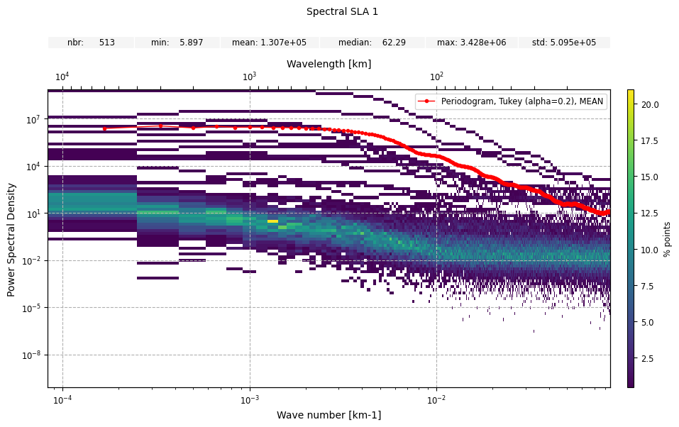
To show the individual psds (psd on each selected segment), add a plot with the parameter individual set to True.

For this plot type, a new parameter, n_bins_psd, will determine the number of bins along the psd values axis (Default: 100).

plot1 = CasysPlot(
    data=ad,
    data_name="Spectral SLA 1",
    plot="psd",
    spectral_name="Periodogram, Tukey (alpha=0.2)",
    plot_params=PlotParams(marker_style="o", marker_size=3, color="red"),
    second_axis=True,
)
plot1.add_stat_bar()

plot2 = CasysPlot(
    data=ad,
    data_name="Spectral SLA 1",
    plot="psd",
    spectral_name="Periodogram, Tukey (alpha=0.2)",
    individual=True,
    n_bins_psd=100,
)
plot1.add_plot(plot2)

plot1.show()

Swath Data

Spectral analysis diagnostics are added using the add_spectral_analysis() method.

Add the computation of a spectral analysis diagnostic.

Spectral analysis data and plots can be accessed or created
using special keywords:

 * plot="psd" (default): Power spectral density along the wave number,
 * plot="segments": Cartographic representation of the selected segments.

The ``segments_reduction`` parameter needs to be provided if more than one
reduction was requested or if computed using dask (the ``stat`` keyword might
be used instead):

 * segments_reduction="mean"
 * segments_reduction="median"

The ``pixel`` parameter needs to be provided to indicate which pixel to use:

 * pixel=20
 * pixel=(55, 60)

Additional plotting options are available to the "psd" plot type:

 * individual: setting it to ``True`` (Default: ``False``) display the set of
   psd on each segments instead of the average psd,
 * n_bins_psd: integer determining the number of bins along the psd values
   axis for the individual=True case (Default: 100),
 * second_axis: flag allowing the display of the second x-axis, for the
   segment length values equivalent to the wave number.

Parameters
----------
name
    Name of the diagnostic.
field
    Field on which to compute the analysis.
segment_length
    Length of a segment (section) in number of points.
    It should be something like a few hundred points. (Example: 500 units)
holes_max_length
    Maximum length of a hole.
    It should be something like a few points (Example: 5)
global_resampling
    Resampling Flag (Default: False).
    True - If one section requires to be resampled => resample all sections.
    False - Resample only  sections requiring a resampling.
delta_t
    Time gap between two measurements.
noise_amplitude
    Noise amplitude in data.
    Default to half of the data standard deviation.
insulation_level
    Minimum valid values percentage on both sides of the hole (Default: 0.75).
    Left and right sides are equal to hole length.
last_segment_overlapping
    Percentage of overlap for second-to-last segment (Default: 0.5).
    When the section is divided in equal segments, the last segment might be
    too short, so it will take some part of data (amount depending on this
    parameter) from the previous segment.
max_time_dispersion
    Maximum allowed percentage of dispersion for delta_t (Default: 5).
    If delta_t dispersion exceed this threshold, a warning will be displayed.
max_resampling
    Maximum resampled data percentage (Default: 0.25).
    A warning will be displayed if this threshold is exceeded.
    The resampling of a large amount of data can have a great impact on the
    final result.
segments_nb_delta_t
    Number of segments used to compute the average time gap between two
    measurements, during the segments extraction process (Default: 1).
segments_nb_delta_x
    Number of segments used to compute the average distance between two
    measurements, during the segments extraction process (Default: 1).
spectral_conf
    Dictionary of the spectral parameters to use for the spectral curve types.
    Each key represents a spectral analysis name is associated with a dictionary
    containing the parameters. This dictionary must contain at least the
    "spectral_type" key and value. (Default: dictionary containing
    the default "periodogram" parameters:
    {"periodogram": {"spectral_type": "periodogram",
    "window": "hann", "detrend": "linear",  ...}}).
segments_reduction
    List of statistic types used to reduce the spectral data across segments
    (Default: mean).
pixels
    Pixels indexes along cross track distance dimension for which to
    compute the diagnostic.
    Either a single integer (for a single pixel) or a list/tuple of:
    - integers: pix
    - list/tuple of two integers, describing a range (pix_min, pix_max)
pixels_selection
    Mode of spectral data reduction for the different spectral curves
    computed for the provided pixel values (Default: "all").
    "all": reduce all the spectral curves for the reduction.
    "range": reduce the spectral curves within a cross track distance range.
    "none": no reduction performed.
pixels_reduction
    Statistic type used to reduce the spectral data across pixels
    (Default: mean).
res_segments
    Flag indicating whether to save the segments data
    in the spectral analysis result (Default: False).
    True - Saving segments data.
    False - Not saving segments data.
res_individual_psd
    Flag indicating whether to save the individual
    power spectrum data on each segments
    in the spectral analysis result (Default: False).
    True - Saving the individual psd data.
    False - Not saving the individual psd data.

This kind of diagnostic can generate 2 kind of plots:

raw data diagnostics map plots for segments selected for the spectral analysis

spectral power density curves plots

Diagnostic setting

In the following example we are setting a spectral analysis diagnostic for the user defined field swh_karin.

from casys import Field

var_swh = Field(
    name="swh_karin",
    unit="m",
)

sd.add_spectral_analysis(
    name="Spectral SWH",
    field=var_swh,
    segment_length=1024,
    holes_max_length=64,
    pixels=[20, 49, [55, 60]],
    spectral_conf={
        "Periodogram, Tukey (alpha=0.2)": {
            "spectral_type": "periodogram",
            "detrend": "linear",
            "window": ("tukey", 0.2),
        },
    },
    pixels_selection="range",
    pixels_reduction="mean",
    res_segments=True,
    res_individual_psd=True,
)

ad.compute()

Diagnostic plotting

Plotting options are identical to NadirData diagnostic case, apart from one additional parameter: pixel.

This parameter allows to specify a pixel value among those provided with the pixels for the diagnostic setting.

Segments plotting

Segments diagnostics are plotted as raw data diagnostics map plots.

plot = CasysPlot(
    data=sd,
    data_name="Spectral SWH",
    plot="segments",
    pixel=20,
    data_params=DataParams(points_min_radius=0.2),
)

plot.show()

Power Spectral Density plotting

Power spectral density (PSD) plots are used to display the requested spectral curves: using a spectral_name value among the previously provided spectral_names.

A second x-axis displaying the equivalent segment length values can be activated by setting the second_axis parameter to True (Default: ``False``).

from casys import TextParams

plot1 = CasysPlot(
    data=sd,
    data_name="Spectral SWH",
    plot="psd",
    spectral_name="Periodogram, Tukey (alpha=0.2)",
    pixel=20,
    second_axis=True,
)
plot1.add_stat_bar()

plot2 = CasysPlot(
    data=sd,
    data_name="Spectral SWH",
    plot="psd",
    spectral_name="Periodogram, Tukey (alpha=0.2)",
    pixel=49,
)
plot2.add_stat_bar()

plot3 = CasysPlot(
    data=sd,
    data_name="Spectral SWH",
    plot="psd",
    spectral_name="Periodogram, Tukey (alpha=0.2)",
    pixel=[55, 60],
)
plot3.add_stat_bar()

plot3.add_plot(plot2)
plot1.add_plot(plot3)
plot1.show()

To show the individual psds (psd on each selected segment), add a plot with the parameter individual set to True.

For this plot type, a new parameter, n_bins_psd, will determine the number of bins along the psd values axis (Default: 100).

from casys import TextParams
plot1 = CasysPlot(
    data=sd,
    data_name="Spectral SWH",
    plot="psd",
    spectral_name="Periodogram, Tukey (alpha=0.2)",
    pixel=20,
    plot_params=PlotParams(marker_style="o", marker_size=3, color="red"),
    second_axis=True,
)
plot1.add_stat_bar()

plot2 = CasysPlot(
    data=sd,
    data_name="Spectral SWH",
    plot="psd",
    spectral_name="Periodogram, Tukey (alpha=0.2)",
    pixel=20,
    individual=True,
    n_bins_psd=100,
)
plot1.add_plot(plot2)

plot1.show()