Crossovers diagnostics - Nadir
add_crossover_stat()
method of the NadirData() container.field.
the difference between the
fieldvalues of the two arcsthe difference between the
timevalues of the two arcs
field values of the two
arcs:
geographical box diagnostics using the parameters:
statsorgeobox_stats
res_lon
res_lat[optional] along time diagnostics using the parameters:
statsortemporal_stats
temporal_stats_freqtemporal_freq_kwargs: dictionary of additional parameters to pass to the pandas.date_range underlying function
Note
stats parameter allows to set the statistics to compute for
temporal and geobox sub-diagnostics at the same time.geobox_stats and/or temporal_stats are also defined, their value will
be used in priority.
max_time_difference: maximum delta of time between the two arcs,
interp_mode: interpolation mode used to compute the field value at the crossover position.
spline_half_window_size: Half window size of the spline.
jump_threshold: tolerance level of the jumps (holes) in the input data.
Add the computation of the difference between the ascending and
descending arc values at crossovers points. Temporal statistics (by
cycle or day) can be added to the computation.

Values and time delta are computed at each point and requested statistics for
each geographical box. These data are accessible using the requested statistics
name or 'crossover' and 'value' keywords for the time delta and the values at
each crossover point.
Time delta (accessible using the 'crossover' keyword) might contain more points
than the actual field statistics if the field is not defined at some crossovers
points.

Crossovers data and plots can be accessed or created using special keywords:

* delta parameter: cartographic representation of the difference
  between the two arcs

    * delta="field": difference of the field values
    * delta="time": difference of the time values

* stat parameter: geographical box or temporal statistic representation.

    * stat="...": requested statistic

* freq parameter: temporal statistic representation.

    * freq="...": frequency of the requested statistic

Parameters
----------
name
    Name of the diagnostic.
field
    Field for which to compute the statistic.
data
    External data (NadirData) to compute crossovers with.
    This option is used to compute multi-missions crossovers.
max_time_difference
    Maximum delta of time between the two arcs as a string with its unit.
    Any string accepted by pandas.Timedelta is valid.
    i.e. '10 days', '6 hours', '1 min', ...
interp_mode
    Interpolation mode used to compute the field value at the crossover
    position.
    Any value accepted by the 'kind' option of scipy.interpolate.interp1d is
    valid.
    i.e. : 'linear' 'nearest' 'previous' 'next' 'zero' 'slinear' 'quadratic'
    or 'cubic' (includes interpolation splines).
    'smooth' is also valid and uses a smoothing spline from scipy.interpolate.
    UnivariateSpline.
    A noise level in the signal may be specified in this form: 'smooth[0.05]'
    Then, the smoothing factor (s parameter of UnivariateSpline) is computed in
    such a way : smoothing_factor = noise_level^2 * number_of_points
    The s parameter roughly represents the distance between the spline and the
    points on the window. In particular, with s=0, we have an interpolation
    spline, which is not suitable for a noisy signal.
    'smooth' alone uses the default value of the s parameter (not recommended).
    The 'smooth' interpolation mode requires at least three valid values on both
    sides of the intersection point.
spline_half_window_size
    Half window size of the spline.
jump_threshold
    This parameter sets the tolerance level of the jumps (holes) in the input
    data. By definition, a jump is detected between (consecutive) P1 and P2 if
    dist(P1, P2) > jump_threshold * MEDIAN where MEDIAN is the median of the
    distance between all consecutive points. For example, to avoid having
    crossovers inside holes of one measure or more, 1.9 is a suitable value.
stats
    List of statistics to compute (count, max, mean, median, min, std, var,
    mad) for temporal and geobox statistics.
res_lon
    Minimum, maximum and box size over the longitude (Default:  -180, 180, 4).
res_lat
    Minimum, maximum and box size over the latitude (Default:  -90, 90, 4).
box_selection
    Field used as selection for computation of the ``count`` statistic.
    Box in which the box_selection field does not contain any data will be set
    to NaN instead of 0.
geobox_stats
    Statistics included in the geobox diagnostic.
temporal_stats_freq
    List of temporal statistics frequencies to compute.
temporal_stats
    Statistics included in the temporal diagnostic.
temporal_freq_kwargs
    Additional parameters to pass to pandas.date_range underlying function.
computation_split
    Split frequency (day, pass, cycle or any pandas offset aliases) inside
    which crossovers will be computed. Providing None (default) will compute
    crossovers over the whole data.

Raises
------
AltiDataError
    If a data already exists with the provided name.
This kind of diagnostic can generate up to 3 kinds of plots:
raw data diagnostics map plots for time and field differences
along time diagnostics plots
Mono-mission crossovers
Diagnostic setting
sla computing a geographical box diagnostics
with default parameters and an along time diagnostics at
cycle and day frequencies.mean and count statistics are computed
for each of these two diagnostics.from casys import Field
sla = Field(
name="SLA",
source="ORBIT.ALTI - RANGE.ALTI - MEAN_SEA_SURFACE.MODEL.CNESCLS15",
unit="m",
)
ad.add_crossover_stat(
name="Crossover SLA",
field=sla,
max_time_difference="5 days",
stats=["mean", "count"],
temporal_stats_freq=["cycle", "day"],
)
ad.compute()
mean and count statistics are computed for the
geobox sub-diagnostic, and the std and count for the temporal sub-diagnostic.ad.add_crossover_stat(
name="Crossover SLA",
field=sla,
max_time_difference="5 days",
geobox_stats=["mean", "count"],
temporal_stats=["std", "count"],
temporal_stats_freq=["cycle", "day"],
)
temporal_freq_kwargs parameter allows to
pass additional parameters to the pandas.date_range underlying function, for custom
frequency values.ad.add_crossover_stat(
name="Crossover SLA",
field=sla,
max_time_difference="5 days",
geobox_stats=["mean", "count"],
temporal_stats=["std", "count"],
temporal_stats_freq=["1H"],
temporal_freq_kwargs={"normalize": True}
)
Diagnostic plotting
CasysPlot uses 3 parameters to determine
what to plot:
delta: plots time or field differences at crossovers
delta= “field”
dela= “time”
stat: plots geographical box diagnostics
stat+freq: plots along time diagnostics
Field and time differences at crossovers
Note
Time differences might contain more points than field differences if the field is not defined at some crossover points.
from casys import CasysPlot

plot = CasysPlot(data=ad, data_name="Crossover SLA", delta="time")

plot.show()

plot = CasysPlot(data=ad, data_name="Crossover SLA", delta="field")

plot.show()

Along time diagnostics
plot = CasysPlot(data=ad, data_name="Crossover SLA", freq="day", stat="mean")

plot.show()

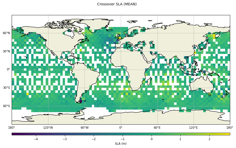
Geographical box diagnostics
plot = CasysPlot(data=ad, data_name="Crossover SLA", stat="mean")

plot.show()
Multi-missions crossovers
data parameter of the
add_crossover_stat() method allows to
calculate crossovers with a second NadirData.Diagnostic setting
Note
The following example compute crossovers between the Jason3 and Sentinel3A missions.
os.environ["GES_TABLE_DIR"] = "/data/cvl_exj3/TABLES/DSC"
ad_j3 = NadirData(
    source="TABLE_C_J3_B",
    orf="C_J3",
    date_start=DateHandler("2021-05-15 12:00:00"),
    date_end=DateHandler("2021-05-17 12:00:00"),
    time="time",
    latitude="LATITUDE",
    longitude="LONGITUDE",
)

ad_s3 = NadirData(
    source="TABLE_C_S3A_B",
    orf="C_S3A",
    date_start=DateHandler("2021-05-15 12:00:00"),
    date_end=DateHandler("2021-05-17 12:00:00"),
    time="time",
    latitude="LATITUDE",
    longitude="LONGITUDE",
)
sig0 = Field(name="SIGMA0_NUMBER.ALTI", unit="m")

ad_j3.add_crossover_stat(
    name="Crossover Sigma 0 J3/S3A",
    field=sig0,
    max_time_difference="5 days",
    data=ad_s3,
)

ad_j3.compute()
Diagnostic plotting
plot = CasysPlot(data=ad_j3, data_name="Crossover Sigma 0 J3/S3A", delta="time")

plot.show()
