Missing points diagnostics
add_missing_points_stat() method.
geographical box diagnostics using the parameters:
geobox_stats= True
res_lon
res_lat[optional] along time diagnostics using the parameters:
temporal_stats_freqtemporal_freq_kwargs: dictionary of additional parameters to pass to the pandas.date_range underlying function
section_min_lengths: list of missing sections minimum length values
group_names, group_grid and group_converter parameters,
add_missing_points_stat() allows to
differentiate results and compute diagnostics for each group in addition to the global
computation.Add the computation of missing points.
Missing points data and plots can be accessed or created using special keywords:
* plot parameter:
* plot="map" (default): along track data
* plot="temporal": temporal statistics data
* plot="geobox": geobox statistics data
* plot="section_analyses": section analyses data
* freq parameter (required for temporal):
* freq="...": frequency of the requested statistic
* dtype parameter:
* dtype="all": data from missing and available points
* dtype="missing" (default): data limited to missing points
* dtype="available": data limited to available points
* group parameter:
* group="global" (default): data from all groups
* group="...": data from the group defined in the group_names parameter.
* sections analyses parameter (optional for section analysis plot):
* sections="all" (default): data from all sections
* sections=1: data limited to section 1
* sections=[1, 2, 10, 14]: data limited to sections 1, 2, 10 and 14
Parameters
----------
name
Name of the diagnostic.
reference_track
File path or data of the reference track.
A list of existing theoretical reference tracks can be shown using the
show_theoretical_tracks method:
>>> CommonData.show_theoretical_tracks()
Standard along track data (orbits) can be provided as well.
This parameter can be provided as a dictionary containing 'data', 'path'
and 'coordinates' keys.
theoretical_orf
ORF to use to determine the real starting and ending dates of the passes.
Using table's ORF might not show missing points in the beginning and end of
a track as well as points for completely missing tracks.
This parameter might not be necessary if using fully defined tracks
(not a theoretical track) as reference.
method
Real: The real method will use the time difference between two real
measurements to determine the missing points.
Theoretical: The theoretical method will try to match each theoretical
points to a real points and use it to determine missing points.
distance_threshold
Distance threshold between real and theoretical points expressed as a factor
of the distance between two consecutive theoretical points.
An exception is raised if the threshold is exceeded.
time_gap_reference
Standard time gap between two consecutive real points.
Use the reference track time gap as default value.
If provided as a string include the unit otherwise it will be considered as
nanoseconds.
time_gap_threshold
[real method parameter] Time threshold between two consecutive real points
expressed as a factor of time_gap_reference to determine that a point is
missing.
The standard value is 2.0: if two consecutive real points have a time gap
of 2.1 * time_gap_reference then a point is considered to be missing.
geobox_stats:
Whether to compute geographical box statistics or not.
res_lon
Minimum, maximum and box size over the longitude (Default: -180, 180, 4)
res_lat
Minimum, maximum and box size over the latitude (Default: -90, 90, 4)
temporal_stats_freq
List of temporal statistics frequencies to compute.
temporal_freq_kwargs
Additional parameters to pass to pandas.date_range underlying function.
section_min_lengths
List of missing sections minimum length values.
Setting this parameter enables the section analyses computation.
group_names
Dictionary containing the name of the group associated to its flag value(s).
Multiple values can be associated to a name.
Example: {"land": 0, "ocean": 1, "ice": 2, "iced_ocean": [1, 2]}.
group_grid
* If True:
* Define two groups {"land": 0, "ocean": 1} using a 1/30 of degree
bathymetry grid file. This method makes the assumption bathymetry
values lesser than 0 are ocean's surface which is not 100% correct.
* If an InGridParameters:
* Define groups using the provided parameters in association with the
group_names parameter.
* If False or None:
* Does not define groups.
group_converter
Callable to apply to grid values to transform them into group values.
This callable has to take a numpy array as single parameter and return a new
one.
If set to None, no conversion is made.
This kind of diagnostic can generate up to 3 kinds of plots:
raw data diagnostics map plots
along time diagnostics plots
Diagnostic setting
J3 reference track, the JA3_ORF CNES ORF and computing along time and
geographical diagnostics.ad.add_missing_points_stat(
name="Missing points 1",
reference_track="J3",
theoretical_orf="JA3_ORF",
geobox_stats=True,
temporal_stats_freq=["pass"],
group_grid=True,
)
ad.compute()
ad.add_missing_points_stat(
    name="Missing points 2",
    reference_track="J3",
    theoretical_orf="JA3_ORF",
    group_grid=True,
    section_min_lengths=[16, 64],
)

ad.compute()
Diagnostic plotting
CasysPlot uses 5 parameters to determine
what to plot:
plot: plot’s type
plot= “map”
plot= “temporal”
plot= “geobox”
dtype:
dtype= “all”: data from missing and available points
dtype= “missing” (default): data limited to missing points
dtype= “available”: data limited to available points
group:
group=”global” (default): data from all groups
group= “…”: data from the group defined in the group_names parameter.
freq: required for temporal
freq= “…”: frequency of the requested statistic
section_min_length: minimal length value of the section analysis to display
sections: optional, for section analyses
sections= “all” (default): show all sections
sections= 1: Number of the section to show
sections= [1 , 4, 10]: List of numbers of sections to show
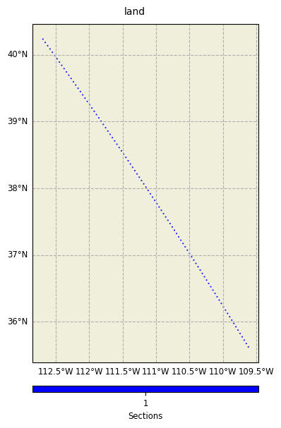
Map plot
from casys import CasysPlot

plot = CasysPlot(
    data=ad,
    data_name="Missing points 1",
    plot="map",
    dtype="missing",
    group="land",
)

plot.show()

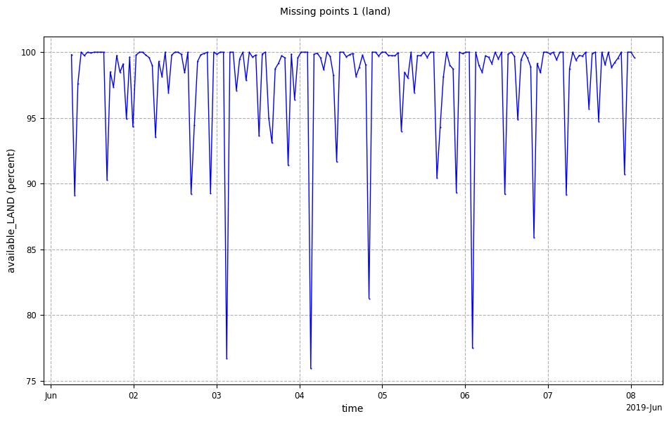
Along time diagnostics
plot = CasysPlot(
    data=ad,
    data_name="Missing points 1",
    plot="temporal",
    freq="pass",
    dtype="available",
    group="land",
)

plot.show()
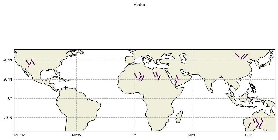
Geographical box diagnostics
plot = CasysPlot(
    data=ad,
    data_name="Missing points 1",
    plot="geobox",
    dtype="available",
    group="land",
)

plot.show()

Section analyses diagnostics
section_min_length=64 section analysis.plot = CasysPlot(
data=ad,
data_name="Missing points 2",
group="global",
plot="section_analyses",
section_min_length=64,
)
plot.show()
section_min_length=16
section analysis.plot = CasysPlot(
data=ad,
data_name="Missing points 2",
plot="section_analyses",
group="land",
section_min_length=16,
)
plot.show()

section_min_length=16
section analysis.plot = CasysPlot(
data=ad,
data_name="Missing points 2",
plot="section_analyses",
group="land",
section_min_length=16,
sections=1,
)
plot.show()