Raw comparison diagnostics

Raw data can be compared against each other using the add_raw_comparison() method and its associated plot.

This diagnostic can be used to compare two x and y fields or three x, y and z fields.

Add a raw data comparison.

In the case of a 3d Raw comparison (z parameter provided), data and plots
can be accessed or created using special keywords:

 * plot="2d" (default): 2d scatter representation.
 * plot="3d": 3d scatter representation.

Parameters
----------
name
    Name of the diagnostic.
x
    Field used for the x-axis.
y
    Field used for the y-axis.
z
    Field used for the z-axis. Optional

Raises
------
AltiDataError
    If a diagnostic already exists with the provided name.

Diagnostic setting

In the following example we are setting a raw comparison diagnostic allowing to visualize:

• SLA values in function of their latitude, for the NadirData.

sla = Field(
    name="SLA",
    source="ORBIT.ALTI - RANGE.ALTI - MEAN_SEA_SURFACE.MODEL.CNESCLS15",
    unit="m",
)
latitude = ad.fields["LATITUDE"]

ad.add_raw_comparison(name="Sla / Latitude", x=latitude, y=sla)

ad.compute()

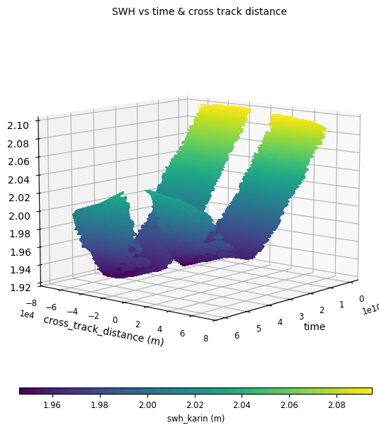
• SWH values in function of the cross_track_distance and time, for a SwathData.

ctd = sd.fields["cross_track_distance"]
time = sd.fields["time"]

sd.add_raw_comparison(
    name="SWH vs time & cross track distance",
    x=time,
    y=ctd,
    z=swh_karin,
)

sd.compute()

Diagnostic plotting

2D plot

(x, y) raw comparison diagnostics are plotted as 2D plots and do not accept any plot parameter:

from casys import CasysPlot

plot = CasysPlot(data=ad, data_name="Sla / Latitude")

plot.show()

For (x, y, z) raw comparison diagnostics, the default plot parameter value is 2d:

from casys import DataParams, DateHandler

x_limits = (
    DateHandler("2014-04-12 15:00:00"),
    DateHandler("2014-04-12 15:01:00"),
)

plot = CasysPlot(
    data=sd,
    data_name="SWH vs time & cross track distance",
    data_params=DataParams(x_limits=x_limits),
)

plot.show()

3D plot

(x, y, z) raw comparison diagnostics have a 3d plotting option available:

x_limits = (
    DateHandler("2014-04-12 15:00:00"),
    DateHandler("2014-04-12 15:01:00"),
)

plot = CasysPlot(
    data=sd,
    data_name="SWH vs time & cross track distance",
    plot="3d:35",
    data_params=DataParams(x_limits=x_limits),
)

plot.show()

In the same way as raw diagnostics, the two swaths of the data can be split using plot="3d:n_pix", with n_pix the index of the splitting pixel.