Binned diagnostics
Binned diagnostics are added using the
add_binned_stat() and
add_binned_stat_2d() methods.Requested statistics will be computed for the
field parameter bands defined by the
x parameter for mono dimensional binned diagnostics or inside boxes defined by the
x and y parameters for two dimensions binned diagnostics.res_x and res_y parameters allows to define the size of band (1D) or box (2D)
in which to compute these statistics.Add a binned diagnostic computing requested statistics inside bands
defined by values of the x parameter according to its resolution.
Parameters
----------
name
Name of the diagnostic.
field
Field on which to compute statistics.
x
Field to use for the x-axis.
stats
List of statistics to compute (count, max, mean, median, min, std, var, mad)
res_x
Min, max and width for the x-axis.
stat_selection
Selection clip used to invalidate (set to NaN) some bins.
Valid conditions are:
* count
* min
* max
* mean
* median
* std
* var
* mad
These clips are Python vector clips.
Examples:
* count :>= 10 && max :< 100
* min :> 3
* median :> 10 && mean :> 9
This kind of diagnostic is plotted as curve plots.
Add a 2D binned diagnostic computing requested statistics inside
boxes defined by values of the x and y parameter according their
respective resolutions.

Binned 2d data and plots can be accessed or created using special keywords:

 * plot="box" (default): color mesh representation, on an x-axis/y-axis grid.
 * plot="curve":

    * axis="x": along x-axis representation of each y-field bin
    * axis="y": along y-axis representation of each x-field bin

 * plot="3d": 3d color mesh representation, on an x-axis/y-axis/z-axis 3d grid.
 * plot="box3d": 3d bins surfaces representation,
   on an x-axis/y-axis/z-axis 3d grid.

Parameters
----------
name
    Name of the diagnostic.
field
    Field on which to compute statistics.
x
    Field to use for the x-axis.
y
    Field to use for the y-axis.
res_x
    Min, max and width for the x-axis.
res_y
    Min, max and width for the y-axis.
stats
    List of statistics to compute (count, max, mean, median, min, std, var, mad)
stat_selection
    Selection clip used to invalidate some bins.
    Valid conditions are:

        * count
        * min
        * max
        * mean
        * median
        * std
        * var
        * mad

    These clips are Python vector clips.
    Examples:

        * count :>= 10 && max :< 100
        * min :> 3
        * median :> 10 && mean :> 9
This kind of diagnostics is plotted as pseudo-color plots with a non-regular rectangular
grid or as a set of curves.
Diagnostic setting
Setting 1D binning
In the following example we are setting a 1D binned diagnostic computing the
mean
of a user defined range_std_ku field inside bands defined by values of the swh
field between 0 and 8 using a 0.05 step.from casys import Field
range_std_ku = Field(
name="range_std_ku",
source="IIF(FLAG_VAL.ALTI==0, RANGE_STD.ALTI, DV)",
unit="m",
)
swh = Field(
name="swh",
source="IIF(FLAG_VAL.ALTI==0, SWH.ALTI, DV)",
unit="m",
)
ad.add_binned_stat(
name="Ku-band range std fct swh",
field=range_std_ku,
x=swh,
res_x=(0, 8, 0.05),
stats=["mean"],
)
ad.compute()
Setting 2D binning
In the following example we are setting a 2D binned diagnostic computing the
median
of a user defined range_std_ku field inside boxes defined by values of the swh
field between 0 and 8 with a 0.05 step and the var_wind field between 0 and 25 with
a 0.5 step.A second 2D binned diagnostic is computed with a lower y-resolution (step of 2.5).
var_wind = Field(
    name="wind",
    source="IIF(FLAG_VAL.ALTI==0, WIND_SPEED.ALTI, DV)",
    unit="m/s",
)

ad.add_binned_stat_2d(
    name="Ku-band range std fct (swh, wind_speed)",
    field=range_std_ku,
    x=swh,
    y=var_wind,
    res_x=(0, 8, 0.05),
    res_y=(0, 25, 0.5),
    stats=["median"],
)

ad.add_binned_stat_2d(
    name="Ku-band range std fct (swh, wind_speed) [2]",
    field=range_std_ku,
    x=swh,
    y=var_wind,
    res_x=(0, 8, 0.05),
    res_y=(0, 25, 2.5),
    stats=["median"],
)

ad.compute()
Diagnostic plotting
Plotting 1D binning
1D binned diagnostics are plotted as curve plots.
CasysPlot requires a stat parameter to
be given in order to know which statistic to display.from casys import CasysPlot
plot = CasysPlot(
data=ad,
data_name='Ku-band range std fct swh',
stat="mean",
)
plot.show()

Plotting 2D binning
2 types of plot are available for the 2D binned diagnostics:
pseudo-color plots (default)
set of curves representing the different y-field bins.
CasysPlot requires a stat parameter to
be given in order to know which statistic to display and an optional plot parameter
indicating the type of plot to use.Pseudo-color plots
2D binned diagnostics can be plotted as pseudo-color plots with a non-regular
rectangular grid by providing the “box” value to the
plot parameter of the
CasysPlot object.Note
This is the default value and not providing the
plot parameter has
the same effect.Low resolution binning
plot = CasysPlot(
    data=ad,
    data_name='Ku-band range std fct (swh, wind_speed) [2]',
    stat="median",
    plot="box",
)

plot.show()

High resolution binning
plot = CasysPlot(
    data=ad,
    data_name="Ku-band range std fct (swh, wind_speed)",
    stat="median",
    plot="box",
)

plot.show()

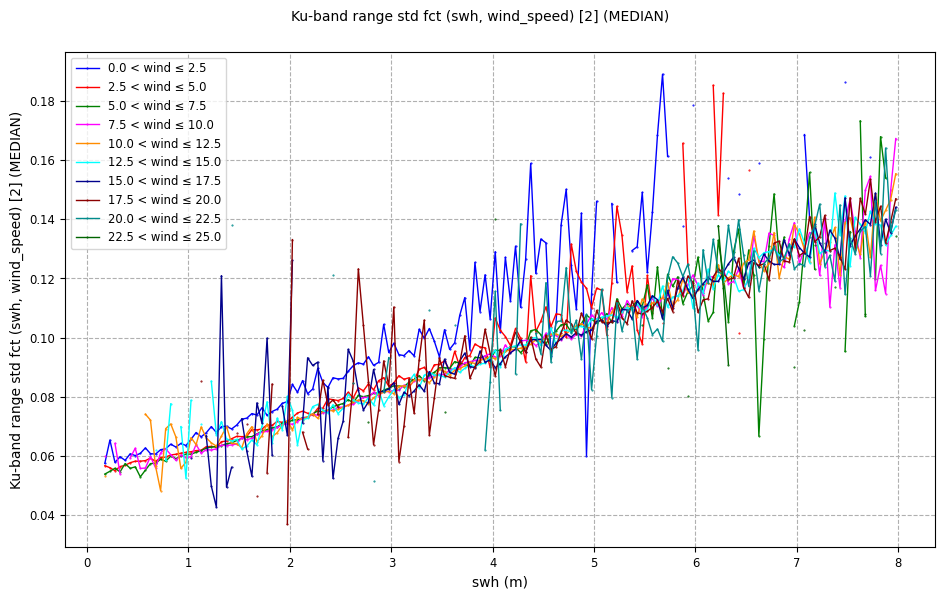
Set of curves
2D binned diagnostics can be plotted as a set of curves with each curve
representing a bin of the
y field.This type of plot is created by providing the “curve” value to the
plot
parameter of the CasysPlot object.Low resolution binning
plot = CasysPlot(
    data=ad,
    data_name='Ku-band range std fct (swh, wind_speed) [2]',
    stat="median",
    plot="curve",
)

plot.show()
Warning
This type of plot might become difficult to read if the resolution of the
y-field is too high and creates a large number of bins/curves.
High resolution binning
plot = CasysPlot(
    data=ad,
    data_name="Ku-band range std fct (swh, wind_speed)",
    stat="median",
    plot="curve",
)

plot.show()

3D plot
2D binned diagnostics can be plotted as a 3d surface.
This type of plot is created by providing the “3d” value to the
plot
parameter of the CasysPlot object.plot = CasysPlot(
data=ad,
data_name="Ku-band range std fct (swh, wind_speed)",
stat="median",
plot="3d",
)
plot.show()

Another 3D plot option is available for 2D binned diagnostics, allowing
to display each bin as a separate surfaces, with box3d.
plot = CasysPlot(
    data=ad,
    data_name="Ku-band range std fct (swh, wind_speed)",
    stat="median",
    plot="box3d",
)

plot.show()
