Click here to download this notebook.

Geographical box statistics

[2]:

from cartopy import crs as ccrs
from casys.readers import CLSTableReader

from casys import CasysPlot, DataParams, DateHandler, Field, NadirData, PlotParams

NadirData.enable_loginfo()

[3]:

# Reader definition
table_name = "TABLE_C_J3_B_GDRD"
start = DateHandler("2019-06-01 05:30:29")
end = DateHandler("2019-06-07 05:47:33")

reader = CLSTableReader(
    name=table_name,
    date_start=start,
    date_end=end,
    time="time",
    longitude="LONGITUDE",
    latitude="LATITUDE",
)

# Data container definition
ad = NadirData(source=reader)

var_swh = Field(name="swh", source="IIF(FLAG_VAL.ALTI == 0, SWH.ALTI, DV)", unit="m")

var_sla = Field(
    name="sla",
    source="ORBIT.ALTI - RANGE.ALTI - MEAN_SEA_SURFACE.MODEL.CNESCLS15",
    unit="m",
)

var_sel = Field(name="box_sel", source="IIF(FLAG_VAL.ALTI == 0, 1, DV)")

We define geobox diagnostics of the SWH and SLA variables including count, mean (or median) and std statistics, using the add_geobox_stat method:

[4]:

# Statistics definition and calculation
ad.add_geobox_stat(
    name="SWH box stat",
    field=var_swh,
    stats=["count", "mean", "std"],
    res_lon=(-180, 180, 2),
    res_lat=(-90, 90, 2),
    box_selection=var_sel,
)

ad.add_geobox_stat(
    name="SLA box stat",
    field=var_sla,
    stats=["count", "median", "std"],
    res_lon=(-180, 180, 2),
    res_lat=(-90, 90, 2),
    box_selection=var_sel,
)

ad.add_raw_data(name="SLA", field=var_sla)

ad.compute()

2025-05-14 10:56:45 INFO    Reading ['LONGITUDE', 'LATITUDE', 'sla', 'time', 'swh', 'box_sel_289cac0f-8095-486d-aab0-50314e7e8ad4', 'box_sel_6e17dd55-389c-4482-85b8-945071c62201']
2025-05-14 10:56:48 INFO    Computing diagnostics ['SWH box stat']
2025-05-14 10:56:48 INFO    Computing diagnostics ['SLA box stat']
2025-05-14 10:56:48 INFO    Computing done.

Plotting SWH box statistic on a map

We specify plot parameters to customize the plot:

[5]:

myplotparams = PlotParams(
    color_map="plasma",
    color_limits=(0, 6),
    grid=True,
    fill_ocean=False,
    projection=ccrs.PlateCarree(central_longitude=180),
)

We create the plot and add some settings using the set_plot_params method:

[6]:

swh_grid_plot = CasysPlot(data=ad, data_name="SWH box stat", stat="mean")

swh_grid_plot.set_plot_params(myplotparams)
swh_grid_plot.add_hist_bar(position="top")
swh_grid_plot.add_stat_bar(position="top")
swh_grid_plot.add_stat_graph(for_axis="latitude", position="right")
swh_grid_plot.set_title("Jason-3 SWH over cycle 127 (m)")

swh_grid_plot.show()

[6]:

../_images/examples_example_advanced_Gridded_Map_10_0.png

Doing the same for the count statistic:

[7]:

myplotparams = PlotParams(
    color_map="plasma",
    color_limits=(0, 90),
    grid=True,
    fill_ocean=False,
    projection=ccrs.PlateCarree(central_longitude=180),
)

swh_grid_plot = CasysPlot(ad, "SWH box stat", stat="count")

swh_grid_plot.set_plot_params(myplotparams)
swh_grid_plot.add_hist_bar(position="top")
swh_grid_plot.add_stat_bar(position="top")
swh_grid_plot.add_stat_graph(for_axis="latitude", position="right")
swh_grid_plot.set_title("Jason-3 SWH over cycle 127 (m)")

swh_grid_plot.show()

[7]:

../_images/examples_example_advanced_Gridded_Map_12_0.png

Using a different projection:

[8]:

myplotparams = PlotParams(
    color_limits=(0, 6),
    grid=True,
    fill_ocean=False,
    projection=ccrs.AlbersEqualArea(central_longitude=180),
)

swh_grid_plot = CasysPlot(data=ad, data_name="SWH box stat", stat="mean")

swh_grid_plot.set_plot_params(myplotparams)
swh_grid_plot.add_hist_bar(position="top")
swh_grid_plot.add_stat_bar(position="top")
swh_grid_plot.set_title("Jason-3 SWH over cycle 127 (m)")

swh_grid_plot.show()

[8]:

../_images/examples_example_advanced_Gridded_Map_14_0.png

Plotting SLA box statistic on a map

[9]:

plot_par = PlotParams(
    color_limits=(0, 1),
    grid=True,
    projection=ccrs.PlateCarree(central_longitude=180),
    fill_ocean=False,
    mask_land=True,
)

slabox_plot = CasysPlot(
    data=ad, data_name="SLA box stat", stat="std", plot_params=plot_par
)

slabox_plot.show()

[9]:

../_images/examples_example_advanced_Gridded_Map_16_0.png

Changing plot parameters:

[10]:

plot_par = PlotParams(
    fig_width=6,
    fig_height=6.5,
    x_limits=(10, 30),
    y_limits=(-50, -30),
    color_limits=(0, 0.6),
    color_map="autumn",
    grid=True,
    mask_land=True,
)
slabox_plot.set_plot_params(plot_par)
slabox_plot.show()

[10]:

../_images/examples_example_advanced_Gridded_Map_18_0.png

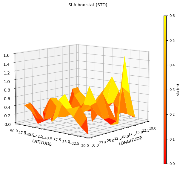
3D plot:

[11]:

slabox_plot = CasysPlot(
    data=ad,
    data_name="SLA box stat",
    stat="std",
    plot="3D",
    plot_params=PlotParams(
        color_map="autumn",
        color_limits=(0, 0.6),
    ),
    data_params=DataParams(
        x_limits=(10, 30),
        y_limits=(-50, -30),
    ),
)

slabox_plot.show()

[11]:

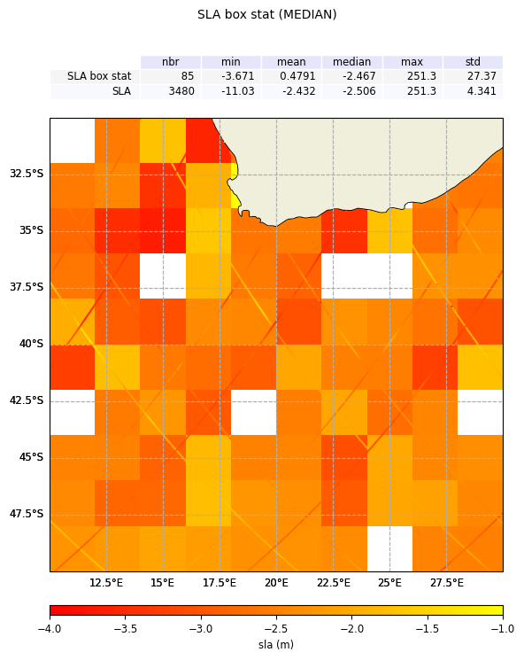
../_images/examples_example_advanced_Gridded_Map_20_0.png

Merging geobox and raw data

Example showing along track SLA with the median geobox SLA over a specific area.

[12]:

slabox_plot_par = PlotParams(
    fig_width=7,
    fig_height=7.5,
    x_limits=(10, 30),
    y_limits=(-50, -30),
    color_limits=(-4, -1),
    color_map="autumn",
    grid=True,
    mask_land=True,
)

data_par = DataParams(x_limits=(10, 30), y_limits=(-50, -30))

slabox_plot = CasysPlot(
    data=ad,
    data_name="SLA box stat",
    stat="median",
    plot_params=slabox_plot_par,
    data_params=data_par,
)

sla_plot_par = PlotParams(color_limits=(-4, -1), color_map="autumn", color_bar=False)

sla_plot = CasysPlot(
    data=ad,
    data_name="SLA",
    plot="map",
    plot_params=sla_plot_par,
    data_params=data_par,
)


slabox_plot.add_stat_bar(position="top")
sla_plot.add_stat_bar(position="top")

slabox_plot.add_plot(sla_plot)

slabox_plot.show()

[12]:

../_images/examples_example_advanced_Gridded_Map_23_0.png