Click here to download this notebook.

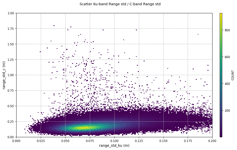
Scatter Ku-band Range std / C-band Range std

from casys import NadirData, CasysPlot, DateHandler, Field, PlotParams
from casys.readers import CLSTableReader

NadirData.enable_loginfo()

Dataset definition

# Reader definition
table_name = "TABLE_C_J3_B_GDRD"
orf_name = "C_J3_GDRD"
cycle_number = 127
start = DateHandler.from_orf(orf_name, cycle_number, 1, pos="first")
end = DateHandler.from_orf(orf_name, cycle_number, 254, pos="last")

reader = CLSTableReader(
    name=table_name,
    date_start=start,
    date_end=end,
    orf=orf_name,
    time="time",
    longitude="LONGITUDE",
    latitude="LATITUDE",
)

# Data container definition
ad = NadirData(source=reader)

var_range_std_ku = Field(
    name="range_std_ku", source="IIF(FLAG_VAL.ALTI==0, RANGE_STD.ALTI,DV)", unit="m"
)
var_range_std_c = Field(
    name="range_std_c", source="IIF(FLAG_VAL.ALTI==0, RANGE_STD.ALTI.B2,DV)", unit="m"
)

Definition of the statistic

Using the add_scatter method:

ad.add_scatter(
    name="Scatter Ku-band Range std / C-band Range std",
    x=var_range_std_ku,
    y=var_range_std_c,
    res_x=(0, 0.2, 0.001),
    res_y=(0, 2, 0.01),
)

Compute

ad.compute()

2025-05-14 10:56:43 INFO    Reading ['range_std_ku', 'range_std_c']
2025-05-14 10:56:46 INFO    Computing diagnostics ['Scatter Ku-band Range std / C-band Range std']
2025-05-14 10:56:46 INFO    Computing done.

Plots

Scatter plot without the regression curve:

disp_plot = CasysPlot(
    data=ad,
    data_name="Scatter Ku-band Range std / C-band Range std",
    plot_params=PlotParams(grid=True, show_reg=False),
)

disp_plot.show()

Scatter plot with the regression curve:

disp_plot = CasysPlot(
    data=ad,
    data_name="Scatter Ku-band Range std / C-band Range std",
    plot_params=PlotParams(grid=True, show_reg=True),
)

disp_plot.show()

Regression curve parameters are available in the data_used attributes of the plot:

• reg_slope

• reg_intercept

• reg_correlation

disp_plot.data_used

<xarray.Dataset> Size: 323kB
Dimensions:       (range_std_ku: 200, range_std_c: 200)
Coordinates:
  * range_std_ku  (range_std_ku) float64 2kB 0.0005 0.0015 ... 0.1985 0.1995
  * range_std_c   (range_std_c) float64 2kB 0.005 0.015 0.025 ... 1.985 1.995
Data variables:
    COUNT         (range_std_ku, range_std_c) int64 320kB 0 0 0 0 0 ... 0 0 0 0
Attributes:
    reg_slope:        1.0671188124867708
    reg_intercept:    0.08997122466706
    reg_correlation:  0.4125913198432696

xarray.Dataset

• Dimensions:
  • range_std_ku: 200
  • range_std_c: 200
• Coordinates: (2)
  • range_std_ku
    (range_std_ku)
    float64
    0.0005 0.0015 ... 0.1985 0.1995

    long_name :

    Box center (x)

    array([0.0005, 0.0015, 0.0025, 0.0035, 0.0045, 0.0055, 0.0065, 0.0075, 0.0085,
           0.0095, 0.0105, 0.0115, 0.0125, 0.0135, 0.0145, 0.0155, 0.0165, 0.0175,
           0.0185, 0.0195, 0.0205, 0.0215, 0.0225, 0.0235, 0.0245, 0.0255, 0.0265,
           0.0275, 0.0285, 0.0295, 0.0305, 0.0315, 0.0325, 0.0335, 0.0345, 0.0355,
           0.0365, 0.0375, 0.0385, 0.0395, 0.0405, 0.0415, 0.0425, 0.0435, 0.0445,
           0.0455, 0.0465, 0.0475, 0.0485, 0.0495, 0.0505, 0.0515, 0.0525, 0.0535,
           0.0545, 0.0555, 0.0565, 0.0575, 0.0585, 0.0595, 0.0605, 0.0615, 0.0625,
           0.0635, 0.0645, 0.0655, 0.0665, 0.0675, 0.0685, 0.0695, 0.0705, 0.0715,
           0.0725, 0.0735, 0.0745, 0.0755, 0.0765, 0.0775, 0.0785, 0.0795, 0.0805,
           0.0815, 0.0825, 0.0835, 0.0845, 0.0855, 0.0865, 0.0875, 0.0885, 0.0895,
           0.0905, 0.0915, 0.0925, 0.0935, 0.0945, 0.0955, 0.0965, 0.0975, 0.0985,
           0.0995, 0.1005, 0.1015, 0.1025, 0.1035, 0.1045, 0.1055, 0.1065, 0.1075,
           0.1085, 0.1095, 0.1105, 0.1115, 0.1125, 0.1135, 0.1145, 0.1155, 0.1165,
           0.1175, 0.1185, 0.1195, 0.1205, 0.1215, 0.1225, 0.1235, 0.1245, 0.1255,
           0.1265, 0.1275, 0.1285, 0.1295, 0.1305, 0.1315, 0.1325, 0.1335, 0.1345,
           0.1355, 0.1365, 0.1375, 0.1385, 0.1395, 0.1405, 0.1415, 0.1425, 0.1435,
           0.1445, 0.1455, 0.1465, 0.1475, 0.1485, 0.1495, 0.1505, 0.1515, 0.1525,
           0.1535, 0.1545, 0.1555, 0.1565, 0.1575, 0.1585, 0.1595, 0.1605, 0.1615,
           0.1625, 0.1635, 0.1645, 0.1655, 0.1665, 0.1675, 0.1685, 0.1695, 0.1705,
           0.1715, 0.1725, 0.1735, 0.1745, 0.1755, 0.1765, 0.1775, 0.1785, 0.1795,
           0.1805, 0.1815, 0.1825, 0.1835, 0.1845, 0.1855, 0.1865, 0.1875, 0.1885,
           0.1895, 0.1905, 0.1915, 0.1925, 0.1935, 0.1945, 0.1955, 0.1965, 0.1975,
           0.1985, 0.1995])

  • range_std_c
    (range_std_c)
    float64
    0.005 0.015 0.025 ... 1.985 1.995

    long_name :

    Box center (y)

    array([0.005, 0.015, 0.025, 0.035, 0.045, 0.055, 0.065, 0.075, 0.085, 0.095,
           0.105, 0.115, 0.125, 0.135, 0.145, 0.155, 0.165, 0.175, 0.185, 0.195,
           0.205, 0.215, 0.225, 0.235, 0.245, 0.255, 0.265, 0.275, 0.285, 0.295,
           0.305, 0.315, 0.325, 0.335, 0.345, 0.355, 0.365, 0.375, 0.385, 0.395,
           0.405, 0.415, 0.425, 0.435, 0.445, 0.455, 0.465, 0.475, 0.485, 0.495,
           0.505, 0.515, 0.525, 0.535, 0.545, 0.555, 0.565, 0.575, 0.585, 0.595,
           0.605, 0.615, 0.625, 0.635, 0.645, 0.655, 0.665, 0.675, 0.685, 0.695,
           0.705, 0.715, 0.725, 0.735, 0.745, 0.755, 0.765, 0.775, 0.785, 0.795,
           0.805, 0.815, 0.825, 0.835, 0.845, 0.855, 0.865, 0.875, 0.885, 0.895,
           0.905, 0.915, 0.925, 0.935, 0.945, 0.955, 0.965, 0.975, 0.985, 0.995,
           1.005, 1.015, 1.025, 1.035, 1.045, 1.055, 1.065, 1.075, 1.085, 1.095,
           1.105, 1.115, 1.125, 1.135, 1.145, 1.155, 1.165, 1.175, 1.185, 1.195,
           1.205, 1.215, 1.225, 1.235, 1.245, 1.255, 1.265, 1.275, 1.285, 1.295,
           1.305, 1.315, 1.325, 1.335, 1.345, 1.355, 1.365, 1.375, 1.385, 1.395,
           1.405, 1.415, 1.425, 1.435, 1.445, 1.455, 1.465, 1.475, 1.485, 1.495,
           1.505, 1.515, 1.525, 1.535, 1.545, 1.555, 1.565, 1.575, 1.585, 1.595,
           1.605, 1.615, 1.625, 1.635, 1.645, 1.655, 1.665, 1.675, 1.685, 1.695,
           1.705, 1.715, 1.725, 1.735, 1.745, 1.755, 1.765, 1.775, 1.785, 1.795,
           1.805, 1.815, 1.825, 1.835, 1.845, 1.855, 1.865, 1.875, 1.885, 1.895,
           1.905, 1.915, 1.925, 1.935, 1.945, 1.955, 1.965, 1.975, 1.985, 1.995])

• Data variables: (1)
  • COUNT
    (range_std_ku, range_std_c)
    int64
    0 0 0 0 0 0 0 0 ... 0 0 0 0 0 0 0 0

    long_name :

    Number of valid pair of values in the box

    array([[0, 0, 0, ..., 0, 0, 0],
           [0, 0, 0, ..., 0, 0, 0],
           [0, 0, 0, ..., 0, 0, 0],
           ...,
           [0, 0, 0, ..., 0, 0, 0],
           [0, 0, 0, ..., 0, 0, 0],
           [0, 0, 0, ..., 0, 0, 0]])

• Indexes: (2)
  • range_std_ku
    PandasIndex

    PandasIndex(Index([               0.0005,                0.0015,                0.0025,
                          0.0035, 0.0045000000000000005,                0.0055,
            0.006500000000000001,                0.0075,                0.0085,
                          0.0095,
           ...
                          0.1905,                0.1915,                0.1925,
                          0.1935,                0.1945,                0.1955,
                          0.1965,                0.1975,                0.1985,
                          0.1995],
          dtype='float64', name='range_std_ku', length=200))

  • range_std_c
    PandasIndex

    PandasIndex(Index([0.005, 0.015, 0.025, 0.035, 0.045, 0.055, 0.065, 0.075, 0.085, 0.095,
           ...
           1.905, 1.915, 1.925, 1.935, 1.945, 1.955, 1.965, 1.975, 1.985, 1.995],
          dtype='float64', name='range_std_c', length=200))

• Attributes: (3)

  reg_slope :

  1.0671188124867708

  reg_intercept :

  0.08997122466706

  reg_correlation :

  0.4125913198432696

To learn more about scatter definition, please visit this documentation page.