Click here to download this notebook.

Binned Statistic with 1D and 2D

[2]:

from casys.readers import CLSTableReader

from casys import CasysPlot, DateHandler, Field, NadirData, PlotParams

NadirData.enable_loginfo()

Dataset definition

[3]:

# Reader definition
table_name = "TABLE_C_J3_B_GDRD"
start = DateHandler("2019-07-20 19:23:06")
end = DateHandler("2019-07-30 17:21:37")

reader = CLSTableReader(
    name=table_name,
    date_start=start,
    date_end=end,
    time="time",
    longitude="LONGITUDE",
    latitude="LATITUDE",
)

# Data container definition
ad = NadirData(source=reader)

var_range_std_ku = Field(
    name="range_std_ku", source="IIF(FLAG_VAL.ALTI==0, RANGE_STD.ALTI,DV)", unit="m"
)
var_swh = Field(name="swh", source="IIF(FLAG_VAL.ALTI==0, SWH.ALTI,DV)", unit="m")
var_wind = Field(
    name="wind", source="IIF(FLAG_VAL.ALTI==0, WIND_SPEED.ALTI, DV)", unit="m/s"
)

Definition of the statistics

Using the add_binned_stat method:

[4]:

ad.add_binned_stat(
    name="Ku-band range std fct swh",
    field=var_range_std_ku,
    x=var_swh,
    res_x=(0, 8, 0.05),
)

ad.add_binned_stat_2d(
    name="Ku-band range std fct (swh, wind_speed)",
    field=var_range_std_ku,
    x=var_swh,
    y=var_wind,
    res_x=(0, 8, 0.05),
    res_y=(0, 25, 0.5),
    stats=["median"],
)

Compute

[5]:

ad.compute()

2025-05-14 10:57:46 INFO    Reading ['swh', 'range_std_ku', 'wind']
2025-05-14 10:57:50 INFO    Computing diagnostics ['Ku-band range std fct swh']
2025-05-14 10:57:50 INFO    Computing diagnostics ['Ku-band range std fct (swh, wind_speed)']
2025-05-14 10:57:50 INFO    Computing done.

Plots

Binned plot with 1 dimension

Binned plot of Ku-band for the mean statistic:

[6]:

rangestd_fctSWH_plot = CasysPlot(
    data=ad,
    data_name="Ku-band range std fct swh",
    stat="mean",
    plot_params=PlotParams(grid=True),
)

rangestd_fctSWH_plot.show()

[6]:

../_images/examples_example_basic_Binned_Statistic_12_0.png

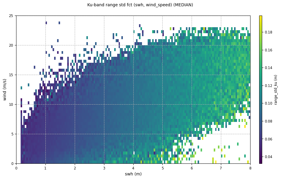
Binned plot with 2 dimensions

Binned plot of Ku-band for the mean statistic with one more dimension:

[7]:

rangestd_fctSWHWind_plot = CasysPlot(
    data=ad,
    data_name="Ku-band range std fct (swh, wind_speed)",
    stat="median",
)

rangestd_fctSWHWind_plot.show()

[7]:

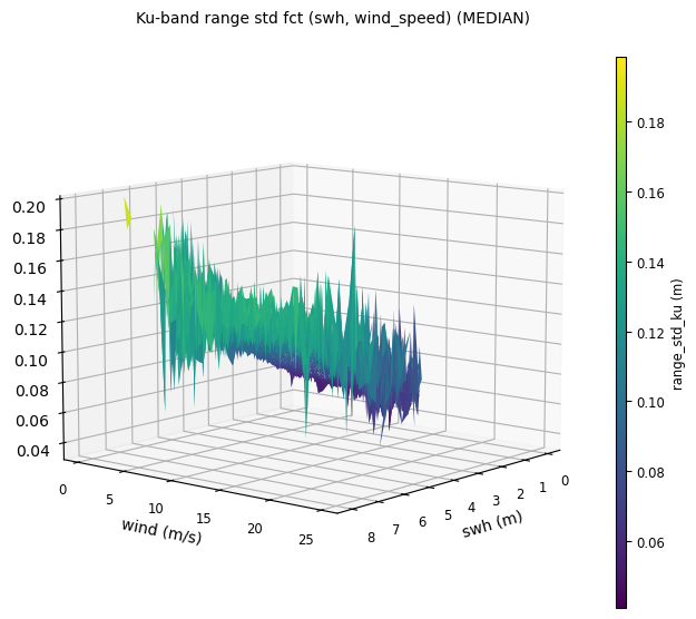
../_images/examples_example_basic_Binned_Statistic_14_0.png

[8]:

rangestd_fctSWHWind_plot = CasysPlot(
    data=ad,
    data_name="Ku-band range std fct (swh, wind_speed)",
    stat="median",
    plot="3d",
)

rangestd_fctSWHWind_plot.show()

[8]:

../_images/examples_example_basic_Binned_Statistic_15_0.png

To learn more about binned diagnostic definition, please visit this documentation page.