Click here to download this notebook.

Missing Points

[2]:

from casys.readers import CLSTableReader

from casys import CasysPlot, DateHandler, NadirData

NadirData.enable_loginfo()

Dataset definition

[3]:

# Reader definition
table_name = "TABLE_C_J3_B_GDRD"
start = DateHandler("2019-07-20 19:23:06")
end = DateHandler("2019-07-30 17:21:37")

reader = CLSTableReader(
    name=table_name,
    date_start=start,
    date_end=end,
    time="time",
    longitude="LONGITUDE",
    latitude="LATITUDE",
)

# Data container definition
ad = NadirData(source=reader)

Definition of the diagnostic

The add_missing_points_stat method allows the definition of a missing points diagnostic.

In the following example we are setting a missing points diagnostic using the default J3 reference track, the C_J3 ORF and computing along time and geographical diagnostics.

In addition, we are using the default grouping parameters allowing to differentiate land and ocean data according to their bathymetry value.

[4]:

ad.add_missing_points_stat(
    name="Missing points",
    reference_track="J3",
    theoretical_orf="C_J3",
    geobox_stats=True,
    temporal_stats_freq=["pass"],
    group_grid=True,
)

2025-05-14 10:55:54 WARNING Computed missing points will be using an ORF build with real measurements. Results might be incomplete.

The section analyses sub-diagnostic setting is shown in this more advanced notebook.

Compute

[5]:

ad.compute()

2025-05-14 10:55:54 INFO    Reading ['time', 'LONGITUDE', 'LATITUDE']
2025-05-14 10:55:57 INFO    Computing diagnostics ['Missing points']
2025-05-14 10:55:57 INFO        Searching missing points.
2025-05-14 10:56:05 INFO    Computing done.

Plot

CasysPlot uses 5 parameters to determine what to plot:

plot: plot’s type (“map”, “temporal”, “geobox”, “section_analyses”)
dtype: “all”, “missing”, “available”
group: “global” (default: data from all groups) or any group defined in the group_names parameter
freq: required for temporal, frequency of the requested statistic
section_min_length: minimal length value of the section analysis to display
sections: optional for section analyses plot

The section analyses sub-diagnostic plotting is shown in this more advanced notebook.

Map plot

Refer to raw data diagnostics documentation for additional information.

Showing missing points on lands:

[6]:

plot = CasysPlot(
    data=ad,
    data_name="Missing points",
    plot="map",
    dtype="missing",
    group="land",
)

plot.show()

[6]:

../_images/examples_example_basic_Missing_Points_15_0.png

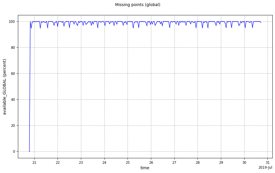
Along time diagnostics

Refer to along time diagnostics documentation for additional information.

Showing percentage of available data:

[7]:

plot = CasysPlot(
    data=ad,
    data_name="Missing points",
    plot="temporal",
    freq="pass",
    dtype="available",
    group="global",
)

plot.show()

[7]:

../_images/examples_example_basic_Missing_Points_18_0.png

Geographical box diagnostics

Refer to geographical box diagnostics documentation for additional information.

Showing available data percentage as geographical boxes:

[8]:

plot = CasysPlot(
    data=ad,
    data_name="Missing points",
    plot="geobox",
    dtype="available",
    group="land",
)

plot.show()

[8]:

../_images/examples_example_basic_Missing_Points_21_0.png

To learn more about missing points definition, please visit this documentation page.