Click here to download this notebook.

Raw data

[2]:

from casys.readers import CLSTableReader

from casys import CasysPlot, DataParams, DateHandler, NadirData, PlotParams

NadirData.enable_loginfo()

Select your data source

[3]:

# Reader definition
table_name = "TABLE_C_J3_B_GDRD"
start = DateHandler("2019-06-01 05:30:29")
end = DateHandler("2019-06-07 05:47:33")

reader = CLSTableReader(
    name=table_name,
    date_start=start,
    date_end=end,
    time="time",
    longitude="LONGITUDE",
    latitude="LATITUDE",
)

# Data container definition
ad = NadirData(source=reader)

Define your diagnostic fields

[4]:

var_sig0 = ad.fields["SIGMA0.ALTI"]

Set up your diagnostic

Using the add_raw_data method:

[5]:

ad.add_raw_data("Sigma 0", var_sig0)

Compute it

[6]:

ad.compute()

2025-05-14 10:59:47 INFO    Reading ['LONGITUDE', 'LATITUDE', 'SIGMA0.ALTI', 'time']
2025-05-14 10:59:49 INFO    Computing done.

Visualize it

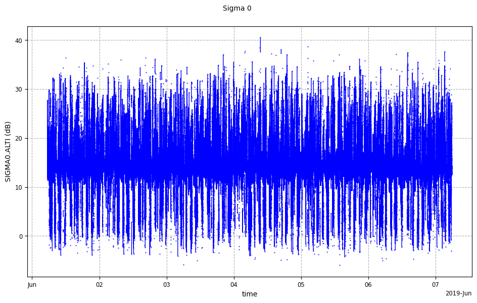
Along time plot of Sigma 0

[7]:

raw_sig0_plot = CasysPlot(ad, "Sigma 0", plot="time")

raw_sig0_plot.show()

[7]:

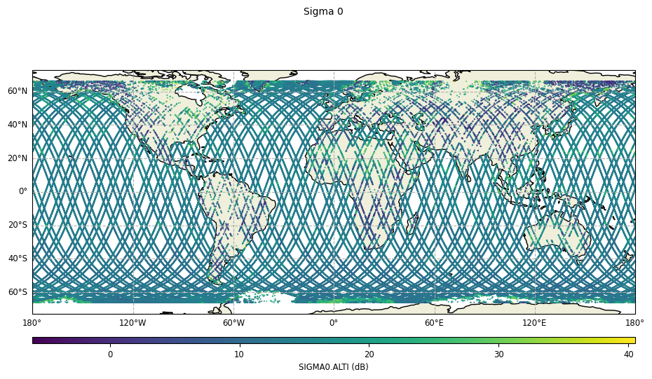
../_images/examples_example_basic_raw_data_14_0.png

Map visualization of Sigma 0

[8]:

sig0_plot = CasysPlot(
    data=ad,
    data_name="Sigma 0",
    plot="map",
)

sig0_plot.show()

[8]:

../_images/examples_example_basic_raw_data_16_0.png

Plots can be customized. Here we define the color limits and y limits parameters, we display a grid and hide lands data using the grid and mask_land parameters.

[9]:

plot_par = PlotParams(
    color_limits=(10, 17), y_limits=(-90, 90), grid=True, mask_land=True
)

sig0_plot = CasysPlot(data=ad, data_name="Sigma 0", plot="map", plot_params=plot_par)

sig0_plot.show()

[9]:

../_images/examples_example_basic_raw_data_18_0.png

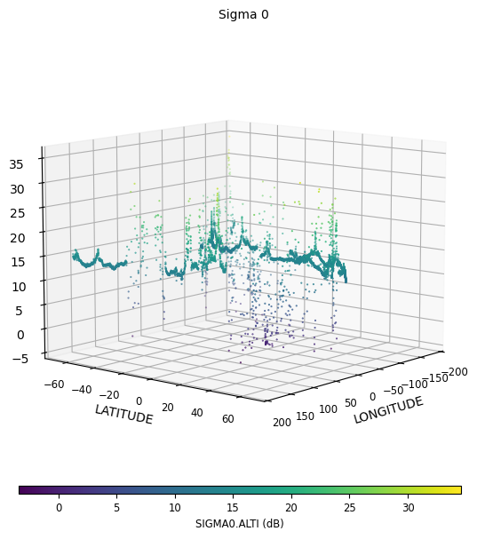
3D visualization of Sigma 0

[10]:

time_limits = ("2019-06-01 15:00:00", "2019-06-01 18:00:00")
sig0_plot = CasysPlot(
    data=ad,
    data_name="Sigma 0",
    plot="3d",
    data_params=DataParams(time_limits=time_limits),
)

sig0_plot.show()

[10]:

../_images/examples_example_basic_raw_data_20_0.png

Additional information about Along track data can be found on this page.