Click here to download this notebook.

Histogram on SLA

[2]:

from casys.readers import CLSTableReader

from casys import CasysPlot, DataParams, DateHandler, Field, NadirData, PlotParams

NadirData.enable_loginfo()

Dataset definition

[3]:

# Reader definition
table_name = "TABLE_C_J3_B_GDRD"
start = DateHandler("2019-07-20 19:23:06")
end = DateHandler("2019-07-30 17:21:37")

reader = CLSTableReader(
    name=table_name,
    date_start=start,
    date_end=end,
    time="time",
    longitude="LONGITUDE",
    latitude="LATITUDE",
)

# Data container definition
ad = NadirData(source=reader)

var_sla = Field(
    name="SLA",
    source="ORBIT.ALTI - RANGE.ALTI - MEAN_SEA_SURFACE.MODEL.CNESCLS15",
    unit="m",
)

Definition of the statistic

The add_histogram method allows the definition of statistics histogram with different res_x resolutions:

[4]:

ad.add_histogram(name="Histo sla", x=var_sla, res_x="auto")

Compute

[5]:

ad.compute()

2025-05-14 10:55:44 INFO    Reading ['SLA']
2025-05-14 10:55:46 INFO    Computing diagnostics ['Histo sla']
2025-05-14 10:55:46 INFO    Computing done.

Plot

Histogram on the SLA

Histogram of the SLA, with bars:

[6]:

sla_hist_plot = CasysPlot(data=ad, data_name="Histo sla")
sla_hist_plot.show()

[6]:

../_images/examples_example_basic_Histogram_12_0.png

Customize the histogram

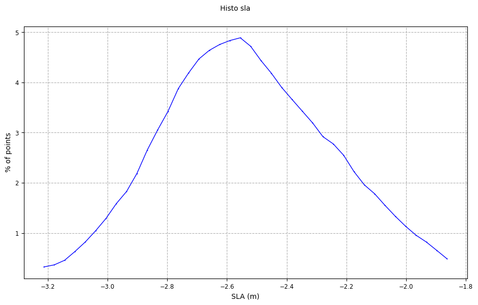
Histogram of the SLA, normalized, without bars, and with grid:

[7]:

sla_hist_plot = CasysPlot(
    data=ad,
    data_name="Histo sla",
    data_params=DataParams(normalize=True),
    plot_params=PlotParams(grid=True, bars=False),
)

sla_hist_plot.show()

[7]:

../_images/examples_example_basic_Histogram_14_0.png

To learn more about histogram definition, please visit this documentation page.