Click here to download this notebook.

Crossover Swath

[2]:

import numpy as np
import swot_calval.io
from casys.readers import ScCollectionReader
from octantng.core.dask import DaskCluster

from casys import CasysPlot, DataParams, PlotParams, SwathData

SwathData.enable_loginfo()

[3]:

dask_cluster = DaskCluster(cluster_type=cluster_type, jobs=(10, 10), memory=4)

dask_client = dask_cluster.client
dask_cluster.wait_for_workers(n_workers=3, timeout=600)

Reader and container definition

Load the crossover table:

[4]:

crossover_table = swot_calval.io.load_crossover_table(
    "/data/OCTANT_NG/tests/ce_swot/swot_science_2015.parquet",
    latitude=80,
    percentage_of_land=15,
)

Initialize the collection reader:

[5]:

collection_path = "/data/OCTANT_NG/tests/ce_swot/zcollection/"

variables = [
    "cross_track_distance",
    "cycle_number",
    "latitude_nadir",
    "latitude",
    "longitude_nadir",
    "longitude",
    "pass_number",
    "time",
    "ssh_karin",
    "swh_karin",
]

reader = ScCollectionReader(
    data_path=collection_path,
    backend_kwargs={
        "cycle_numbers": 10,
        "pass_numbers": np.arange(100),
        "selected_variables":  variables,
    },
    time="time",
    latitude="latitude",
    longitude="longitude",
    latitude_nadir="latitude_nadir",
    longitude_nadir="longitude_nadir",
    cycle_number="cycle_number",
    pass_number="pass_number",
)

[6]:

sd = SwathData(source=reader)

Definition of the crossover diagnostic

Using the add_crossover_stat method:

[7]:

sd.add_crossover_stat(
    name="SSH Crossover",
    field=sd.fields["ssh_karin"],
    stats=["mean", "std"],
    temporal_stats_freq=["1h", "DAY"],
    max_time_difference="10 days",
    crossover_table=crossover_table,
    diamond_relocation=True,
    diamond_reduction="mean",
)

[8]:

sd.add_crossover_stat(
    name="SWH Crossover",
    field=sd.fields["swh_karin"],
    stats=["mean", "std"],
    temporal_stats_freq=["1h", "DAY"],
    max_time_difference="10 days",
    crossover_table=crossover_table,
    diamond_relocation=True,
    diamond_reduction="mean",
)

[9]:

sd.add_crossover_stat(
    name="SWH Crossover no relocation",
    field=sd.fields["swh_karin"],
    stats=["mean", "std"],
    temporal_stats_freq=["1h", "DAY"],
    max_time_difference="10 days",
    crossover_table=crossover_table,
    diamond_relocation=False,
    diamond_reduction="mean",
)

Note The reduction step occurs after computing binning diagnostics.

Computation

The two crossover diagnostic on ssh_karin and swh_karin values will be computed simultaneously (same computation parameters).

[10]:

sd.compute_dask()

2025-05-14 10:58:15 INFO    Computing diagnostics ['SSH Crossover']
2025-05-14 10:59:50 INFO    Computing diagnostics ['SWH Crossover']
2025-05-14 11:01:05 INFO    Computing diagnostics ['SWH Crossover no relocation']
2025-05-14 11:02:21 INFO    Computing done.

Note Crossover diagnostics can be computed without crossover table input, at computation time cost.

Plot

Along time diagnostic

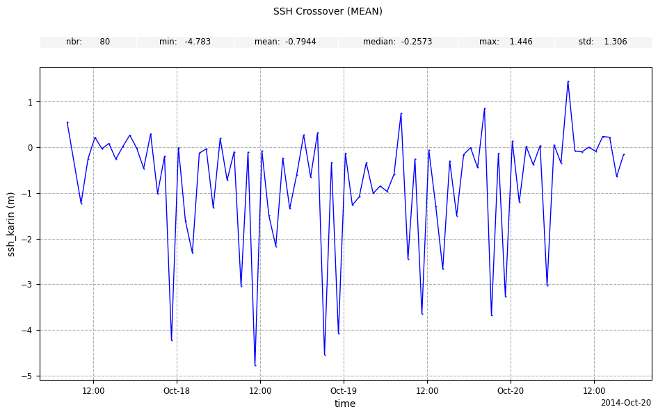
Plot the temporal diagnostic, for a specific statistic and frequency:

mean statistic and 1h frequency for ssh_karin

[11]:

plot_along_time_ssh = CasysPlot(
    data=sd,
    data_name="SSH Crossover",
    stat="mean",
    freq="1h",
    data_params=DataParams(remove_nan=True),
)
plot_along_time_ssh.add_stat_bar()
plot_along_time_ssh.show()

[11]:

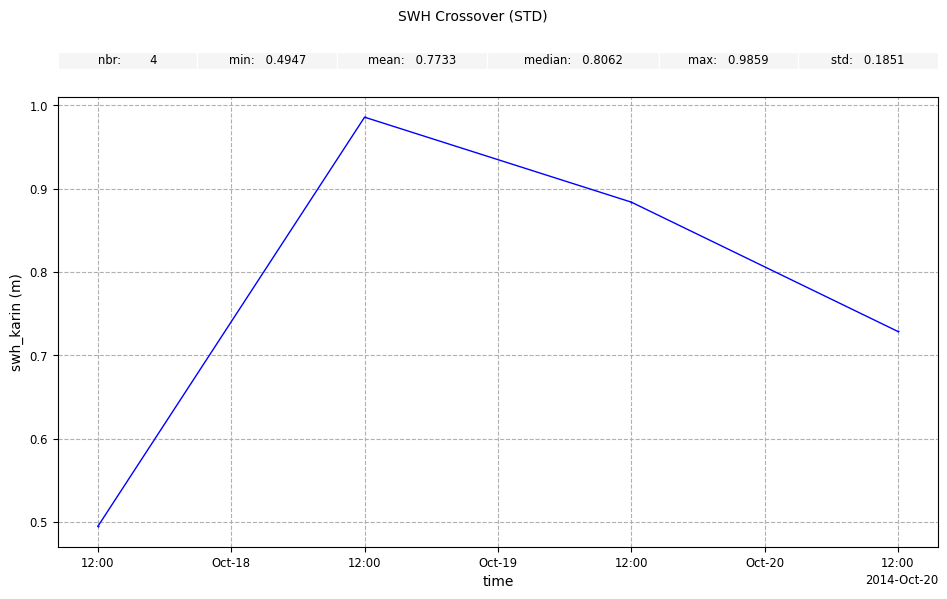
../_images/examples_example_basic_Crossovers_Statistic_Swath_23_0.png

std statistic and DAY frequency for swh_karin

[12]:

plot_along_time_swh = CasysPlot(
    data=sd,
    data_name="SWH Crossover",
    stat="std",
    freq="DAY",
    data_params=DataParams(remove_nan=True),
)
plot_along_time_swh.add_stat_bar()
plot_along_time_swh.show()

[12]:

../_images/examples_example_basic_Crossovers_Statistic_Swath_25_0.png

Geographical box diagnostics

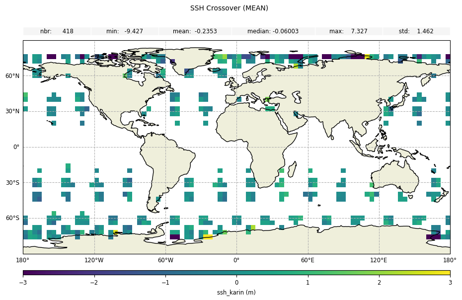
Plot the geobox diagnostics, providing the diagnostic name and a specific statistic:

mean statistic for ssh_karin

[13]:

plot_geobox_mean = CasysPlot(
    data=sd,
    data_name="SSH Crossover",
    stat="mean",
    plot_params=PlotParams(color_limits=(-3, 3)),
)
plot_geobox_mean.add_stat_bar()
plot_geobox_mean.show()

[13]:

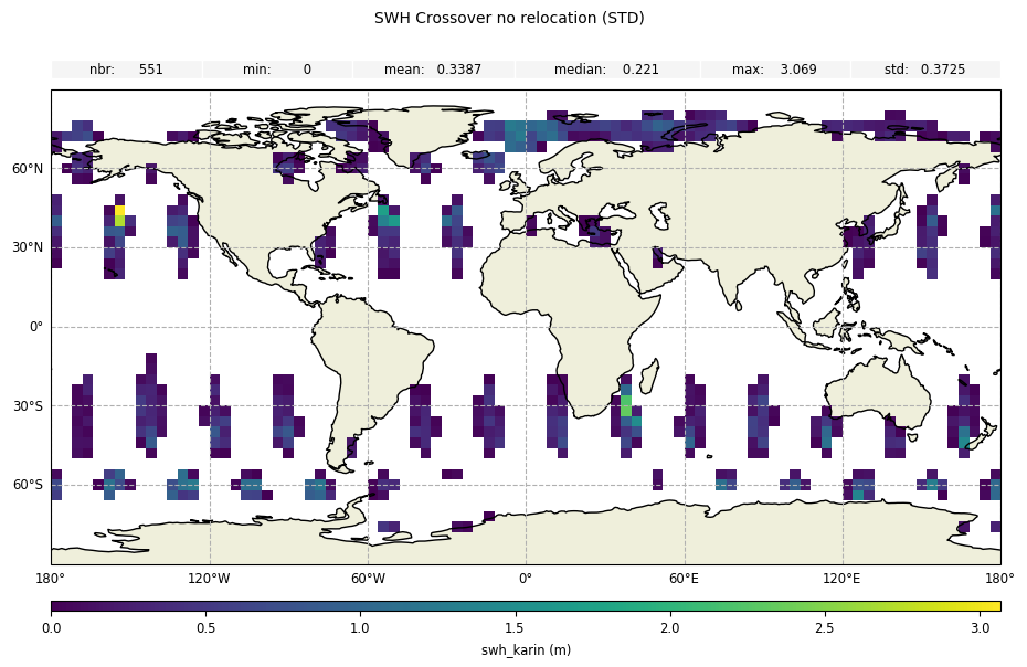
../_images/examples_example_basic_Crossovers_Statistic_Swath_29_0.png

std statistic for swh_karin

[14]:

plot_geobox_std = CasysPlot(
    data=sd,
    data_name="SWH Crossover",
    stat="std",
)
plot_geobox_std.add_stat_bar()
plot_geobox_std.show()

[14]:

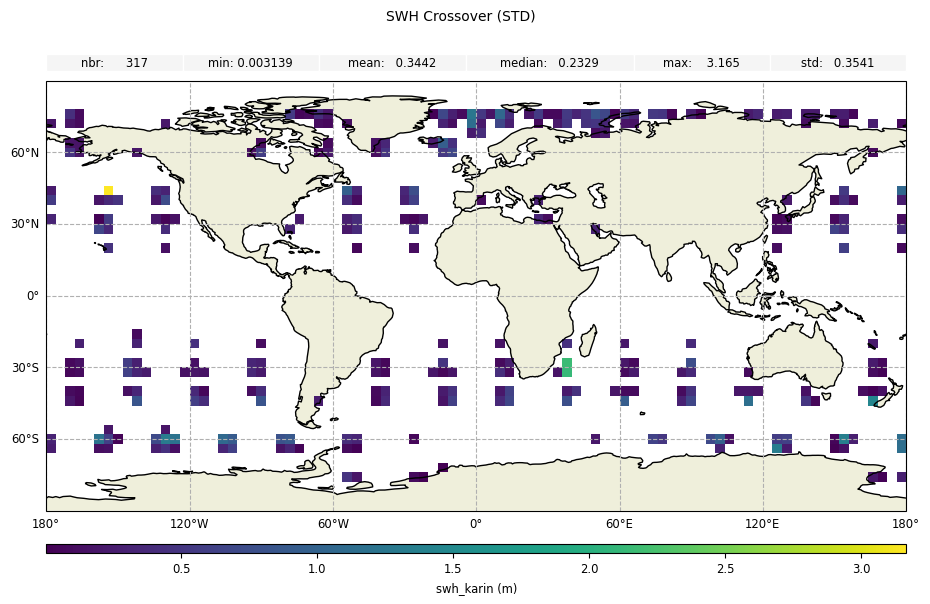
../_images/examples_example_basic_Crossovers_Statistic_Swath_31_0.png

For the crossover diagnostic on swh without diamond relocation, we can notice small differences:

[15]:

plot_geobox_no_reloc = CasysPlot(
    data=sd,
    data_name="SWH Crossover no relocation",
    stat="std",
)
plot_geobox_no_reloc.add_stat_bar()
plot_geobox_no_reloc.show()

[15]:

../_images/examples_example_basic_Crossovers_Statistic_Swath_33_0.png

Field and time differences at crossovers

Plot the time or field value at crossover points (on the full diamonds or at nadir coordinates depending on the diamond_reduction parameter).

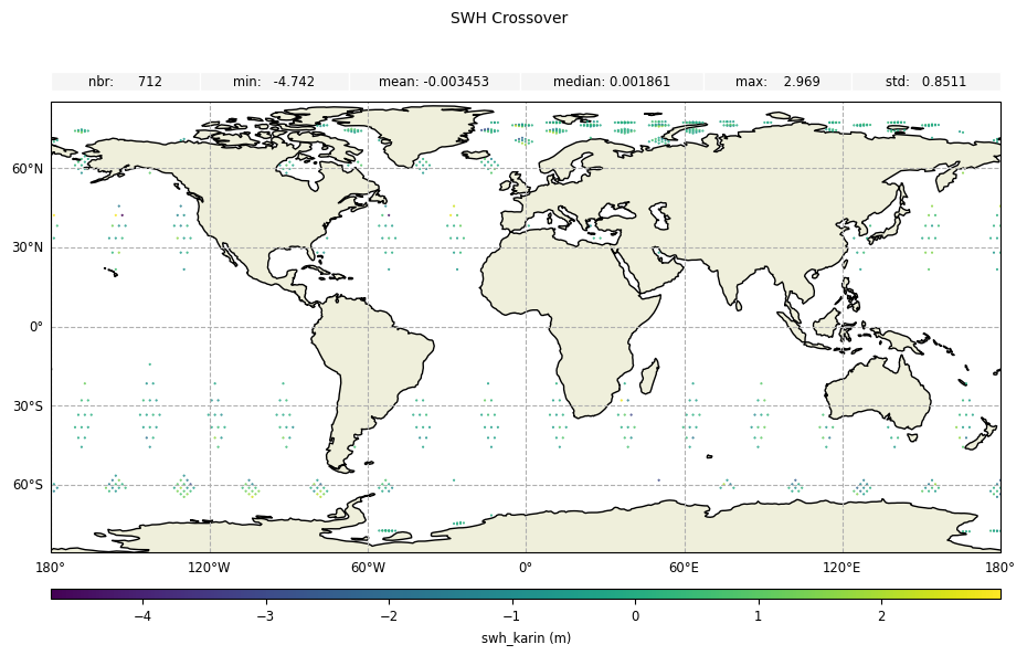
Field delta values

For field values at crossover points. Here diamond_reduction='mean', the field value is the averaged value of the field difference on the crossover diamond.

[16]:

plot_field_delta = CasysPlot(
    data=sd,
    data_name="SWH Crossover",
    delta="field",
)
plot_field_delta.add_stat_bar()
plot_field_delta.show()

[16]:

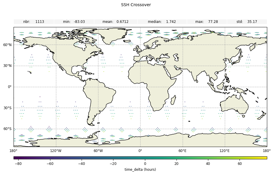
../_images/examples_example_basic_Crossovers_Statistic_Swath_38_0.png

Time delta values

For time difference at crossover points:

[17]:

plot_time_delta = CasysPlot(
    data=sd,
    data_name="SSH Crossover",
    delta="time",
)
plot_time_delta.add_stat_bar()
plot_time_delta.show()

[17]:

../_images/examples_example_basic_Crossovers_Statistic_Swath_41_0.png

Example without crossovers diamond reduction

Query the collection a few passes and repeat the previous steps with diamond_reduction=False for the crossover diagnostic:

Creating SwathData object:

[18]:

reader_part = ScCollectionReader(
    data_path=collection_path,
    backend_kwargs={
        "cycle_numbers": 10,
        "pass_numbers": [1, 154, 2, 155],
        "selected_variables": variables,
    },
    time="time",
    latitude="latitude",
    longitude="longitude",
    latitude_nadir="latitude_nadir",
    longitude_nadir="longitude_nadir",
    cycle_number="cycle_number",
    pass_number="pass_number",
)

[19]:

sd_part = SwathData(source=reader_part)

Adding the crossover diagnostic with diamond_reduction=False:

[20]:

sd_part.add_crossover_stat(
    name="SSH Crossover",
    field=sd_part.fields["ssh_karin"],
    stats="mean",
    max_time_difference="10 days",
    crossover_table=crossover_table,
    diamond_relocation=True,
    diamond_reduction="none",
)

Computing the diagnostic:

[21]:

sd_part.compute()

2025-05-14 11:02:24 INFO    Computing diagnostics ['SSH Crossover']
2025-05-14 11:02:27 INFO    Computing done.

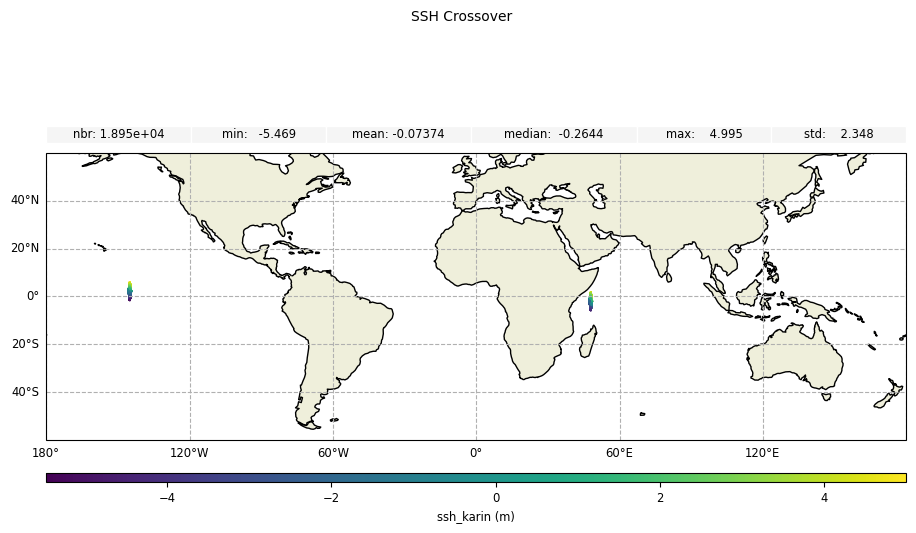
Plot the field value difference for crossover diamond points:

[22]:

plot_field_delta = CasysPlot(
    data=sd_part,
    data_name="SSH Crossover",
    delta="field",
    plot_params=PlotParams(grid=True, y_limits=(-60, 60)),
)
plot_field_delta.add_stat_bar()
plot_field_delta.show()

[22]:

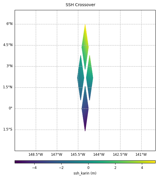
../_images/examples_example_basic_Crossovers_Statistic_Swath_52_0.png

Zoom on a crossover diamond:

[23]:

plot_field_delta = CasysPlot(
    data=sd_part,
    data_name="SSH Crossover",
    delta="field",
    plot_params=PlotParams(grid=True, y_limits=(-3, 7), x_limits=(-150, -140)),
)
plot_field_delta.show()

[23]:

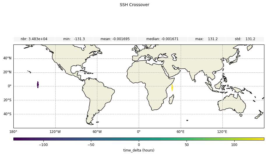
../_images/examples_example_basic_Crossovers_Statistic_Swath_54_0.png

Plot the time difference value for crossover diamond points:

[24]:

plot_time_delta = CasysPlot(
    data=sd_part,
    data_name="SSH Crossover",
    delta="time",
    plot_params=PlotParams(grid=True, y_limits=(-60, 60)),
)
plot_time_delta.add_stat_bar()
plot_time_delta.show()

[24]:

../_images/examples_example_basic_Crossovers_Statistic_Swath_56_0.png

Zoom on another crossover diamond:

[25]:

plot_time_delta = CasysPlot(
    data=sd_part,
    data_name="SSH Crossover",
    delta="time",
    plot_params=PlotParams(grid=True, y_limits=(-8, 4), x_limits=(35, 60)),
)
plot_time_delta.show()

[25]:

../_images/examples_example_basic_Crossovers_Statistic_Swath_58_0.png