Click here to download this notebook.

Periodogram

import numpy as np

from casys import CasysPlot, DateHandler, Field, NadirData
from casys.readers import CLSTableReader

NadirData.enable_loginfo()

Dataset definition

# Reader definition
table_name = "TABLE_C_J3_B_GDRD"
orf_name = "C_J3"
cycle_number = 127
start = DateHandler.from_orf(orf_name, cycle_number, 1, pos="first")
end = DateHandler.from_orf(orf_name, cycle_number, 254, pos="last")

reader = CLSTableReader(
    name=table_name,
    date_start=start,
    date_end=end,
    orf=orf_name,
    time="time",
    longitude="LONGITUDE",
    latitude="LATITUDE",
)

# Data container definition
ad = NadirData(source=reader)

var_swh = Field(name="swh", source="IIF(FLAG_VAL.ALTI==0, SWH.ALTI,DV)", unit="m")
var_sla = Field(
    name="sla",
    source="ORBIT.ALTI - RANGE.ALTI - MEAN_SEA_SURFACE.MODEL.CNESCLS15",
    unit="m",
)

Definition of the statistics

The add_periodogram method allows the computation of periodograms from the result of a temporal diagnostic or sub-diagnostic (from a crossover or missing points diagnostic).

first_period = np.timedelta64(1, "D")
last_period = np.timedelta64(20, "D")
nbr_periods = 64

From a temporal diagnostic

Only the stats is needed to select the correct temporal diagnostic results.

ad.add_time_stat(name="SWH by hour", freq="1h", field=var_swh, stats=["mean", "std"])
ad.add_periodogram(
    name="Periodogram SWH by hour",
    base_diag="SWH by hour",
    stats=["mean", "std"],
    nbr_periods=nbr_periods,
    first_period=first_period,
    last_period=last_period,
)

From a crossover temporal sub-diagnostic

For a crossover temporal sub-diagnostic, more parameters are needed to select the correct sub diagnostic among those computed in the base diagnostic. Those parameter will be provided through the diag_kwargs, with a dictionary.

In the present case, the only kwargs expected in diag_kwargs is the freq value, as several frequencies can be defined for the crossover temporal sub-diagnostic computation (here “cycle” and “pass”, see temporal_stats_freq).

ad.add_crossover_stat(
    name="Crossover SLA",
    field=var_sla,
    max_time_difference="10 days",
    stats=["mean", "count"],
    temporal_stats_freq=["cycle", "pass"],
)
ad.add_periodogram(
    name="Periodogram Crossover SLA by pass",
    base_diag="Crossover SLA",
    stats=["mean", "count"],
    nbr_periods=nbr_periods,
    first_period=first_period,
    last_period=last_period,
    diag_kwargs={"freq": "pass"},
)

From a missing points temporal sub-diagnostic

For a missing points temporal sub-diagnostic, the kwargs expected in diag_kwargs are:

• the freq value, as several frequencies can be defined for the crossover temporal sub-diagnostic computation (here “1h” and “20min”, see temporal_stats_freq),

• the dtype value, “missing”, “available” or “all”,

• the group value, “GLOBAL” or any of the other groups defined with the group_grid parameter (“OCEAN” and “LAND” in the default case group_grid=True)

ad.add_missing_points_stat(
    name="Missing Points",
    reference_track="J3",
    temporal_stats_freq=["1h", "20min"],
    group_grid=True,
)
ad.add_periodogram(
    name="Periodogram Missing Points by hour",
    base_diag="Missing Points",
    stats=["count"],
    nbr_periods=nbr_periods,
    first_period=first_period,
    last_period=last_period,
    diag_kwargs={"freq": "1h", "dtype": "missing", "group": "LAND"},
)

2025-05-14 10:56:13 WARNING Computed missing points will be using an ORF build with real measurements. Results might be incomplete.

Compute

ad.compute()

2025-05-14 10:56:13 INFO    Reading ['time', 'swh', 'LONGITUDE', 'LATITUDE', 'sla']
2025-05-14 10:56:17 INFO    Computing diagnostics ['SWH by hour']
2025-05-14 10:56:17 INFO    Computing diagnostics ['Crossover SLA']
2025-05-14 10:56:19 INFO    Computing diagnostics ['Missing Points']
2025-05-14 10:56:19 INFO        Searching missing points.
2025-05-14 10:56:27 INFO    Computing Periodogram SWH by hour
2025-05-14 10:56:27 INFO    Computing Periodogram Crossover SLA by pass
2025-05-14 10:56:27 INFO    Computing Periodogram Missing Points by hour
2025-05-14 10:56:27 INFO    Computing done.

ad

AltiData
	Source Source type ORF Time name Longitude Latitude	TABLE_C_J3_B_GDRD CLSTableReader C_J3 time LONGITUDE LATITUDE		Period start Period end Selection clip Selection shape	2019-07-20 19:23:06.823509 Cycle: 127 - Pass: 1 2019-07-30 17:21:37.233369 Cycle: 127 - Pass: 254 None False
Time statistics	Name	Field	Frequency		Statistics		State
	SWH by hour	swh	1h		[MEAN, STD]		Computed
Periodogram analysis	Name	Base Diagnostic		Description		Statistics	State
	Periodogram Crossover SLA by pass	Crossover SLA {'freq': 'pass'}		Number of periods: 64 First period: 1 days Last period: 20 days		[MEAN, COUNT]	Computed
	Periodogram Missing Points by hour	Missing Points {'freq': '1h', 'dtype': MISSING, 'group': 'LAND', 'plot': 'temporal'}		Number of periods: 64 First period: 1 days Last period: 20 days		[COUNT]	Computed
	Periodogram SWH by hour	SWH by hour		Number of periods: 64 First period: 1 days Last period: 20 days		[MEAN, STD]	Computed
Crossovers	Name	Description	Fields	Resolution	Frequencies	Statistics	State
	Crossover SLA	Max time difference: 240.0 hours Interpolation mode: linear Spline half window size: 3	sla	Longitude: min: -180, max: 180, step: 4 Latitude: min: -90, max: 90, step: 4	['CYCLE', 'PASS']	Temporal: [MEAN, COUNT] Geobox: [MEAN, COUNT]	Computed
Missing Points	Name		Description		Resolution	Frequencies	State
	Missing Points		Groups: ['GLOBAL', 'LAND', 'OCEAN'] Method: REAL Distance threshold: 4.0 Reference time gap: 1.08 sec Time threshold: 1.9		Longitude: min: -180, max: 180, step: 4 Latitude: min: -90, max: 90, step: 4	['1h', '20min']	Computed

Plot

This diagnostic is plotted as curve, along the periods values computed. We need to provide a stat parameter value to the CasysPlot.

From a temporal diagnostic

periodogram_temporal_plot = CasysPlot(
    data=ad, data_name="Periodogram SWH by hour", stat="std"
)
periodogram_temporal_plot.show()

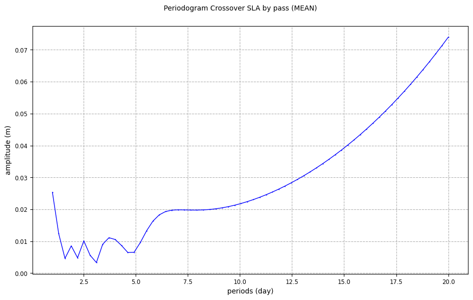
From a crossover temporal sub-diagnostic

periodogram_crossover_plot = CasysPlot(
    data=ad, data_name="Periodogram Crossover SLA by pass", stat="mean"
)
periodogram_crossover_plot.show()

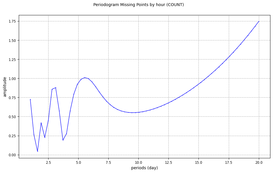
From a missing points temporal sub-diagnostic

periodogram_missingpoints_plot = CasysPlot(
    data=ad, data_name="Periodogram Missing Points by hour", stat="count"
)
periodogram_missingpoints_plot.show()

To learn more about periodogram diagnostic definition, please visit this documentation page.