Click here to download this notebook.

Spectral Analysis - Swath

[2]:

from casys.readers import ScCollectionReader
from octantng.core.dask import DaskCluster

from casys import CasysPlot, DataParams, Field, PlotParams, SwathData

[3]:

dask_cluster = DaskCluster(cluster_type=cluster_type, jobs=(5, 5), memory=8)

dask_client = dask_cluster.client
dask_cluster.wait_for_workers(n_workers=3, timeout=600)

Reader and container definition

[4]:

collection_path = "/data/OCTANT_NG/tests/ce_swot/zcollection/"

reader = ScCollectionReader(
    data_path=collection_path,
    backend_kwargs={"cycle_numbers": 8},
    longitude="longitude",
    latitude="latitude",
)

[5]:

sd = SwathData(source=reader)

Definition of the spectral analysis diagnostic

Using the add_spectral_analysis method:

[6]:

ssh_e = Field(
    name="ssh_karin_w_error",
    source=(
        "simulated_true_ssh_karin + simulated_error_karin + "
        "simulated_error_timing + simulated_error_roll + simulated_error_phase"
    ),
)

[7]:

sd.add_spectral_analysis(
    name="SSH Karin Spectral",
    field=ssh_e,
    segment_length=1024,
    holes_max_length=64,
    res_segments=True,
    res_individual_psd=True,
    pixels=[20, 49, [55, 60]],
    spectral_conf={
        "Periodogram, Tukey (alpha=0.2)": {
            "spectral_type": "periodogram",
            "detrend": "linear",
            "window": ("tukey", 0.2),
        },
    },
    pixels_selection="range",
    pixels_reduction="mean",
)

Computation

[8]:

sd.compute_dask()

2025-05-14 10:57:32 WARNING [SSH Karin Spectral] Spectral analysis provides better results with a 'cycle' or 'pass' compatible frequency.
2025-05-14 10:59:21 WARNING Field 'ssh_karin_w_error' merged spectral analysis results have a 'delta_t' relative standard error of 0.277517%
2025-05-14 10:59:21 WARNING Field 'ssh_karin_w_error' merged spectral analysis results have a 'delta_t' relative standard error of 0.276169%
2025-05-14 10:59:21 WARNING Field 'ssh_karin_w_error' merged spectral analysis results have a 'delta_t' relative standard error of 0.276098%

Plotting

PSD

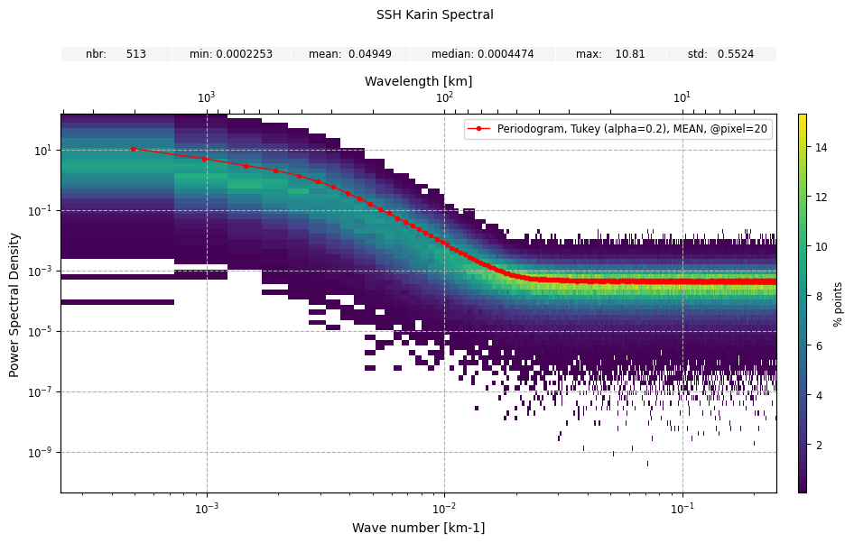
[9]:

plot_psd_1 = CasysPlot(
    data=sd,
    data_name="SSH Karin Spectral",
    plot="PSD",
    plot_params=PlotParams(grid=True),
    spectral_name="Periodogram, Tukey (alpha=0.2)",
    pixel=20,
    second_axis=True,
)
plot_psd_1.add_stat_bar()

plot_psd_2 = CasysPlot(
    data=sd,
    data_name="SSH Karin Spectral",
    plot="PSD",
    plot_params=PlotParams(grid=True, line_style="", marker_size=4),
    spectral_name="Periodogram, Tukey (alpha=0.2)",
    pixel=49,
)
plot_psd_2.add_stat_bar()

plot_psd_3 = CasysPlot(
    data=sd,
    data_name="SSH Karin Spectral",
    plot="PSD",
    plot_params=PlotParams(grid=True, line_style="", marker_size=4),
    spectral_name="Periodogram, Tukey (alpha=0.2)",
    pixel=[55, 60],
)
plot_psd_3.add_stat_bar()

plot_psd_1.add_plot(plot_psd_2)
plot_psd_1.add_plot(plot_psd_3)
plot_psd_1.show()

[9]:

../_images/examples_example_basic_Spectral_Analysis_Swath_15_0.png

[10]:

plot_psd_1 = CasysPlot(
    data=sd,
    data_name="SSH Karin Spectral",
    plot="PSD",
    spectral_name="Periodogram, Tukey (alpha=0.2)",
    pixel=20,
    plot_params=PlotParams(grid=True, marker_style="o", marker_size=3, color="red"),
    second_axis=True,
)
plot_psd_1.add_stat_bar()

plot_psd_2 = CasysPlot(
    data=sd,
    data_name="SSH Karin Spectral",
    plot="PSD",
    plot_params=PlotParams(grid=True),
    spectral_name="Periodogram, Tukey (alpha=0.2)",
    pixel=20,
    individual=True,
    n_bins_psd=75,
)
plot_psd_1.add_plot(plot_psd_2)

plot_psd_1.show()

[10]:

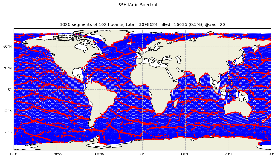
../_images/examples_example_basic_Spectral_Analysis_Swath_16_0.png

SEGMENTS

[11]:

plot_segments = CasysPlot(
    data=sd,
    data_name="SSH Karin Spectral",
    plot="SEGMENTS",
    plot_params=PlotParams(grid=True),
    data_params=DataParams(points_min_radius=0.5),
    pixel=20,
)
plot_segments.show()

[11]:

../_images/examples_example_basic_Spectral_Analysis_Swath_18_0.png

To learn more about spectral analysis diagnostic definition, please visit this documentation page.