Click here to download this notebook.

Temporal evolution of SWH

[2]:

from casys.readers import CLSTableReader

from casys import CasysPlot, DateHandler, Field, NadirData, PlotParams

NadirData.enable_loginfo()

Dataset definition

[3]:

# Reader definition
table_name = "TABLE_C_J3_B_GDRD"
orf_name = "C_J3"
cycle_number = 127
start = DateHandler.from_orf(orf_name, cycle_number, 1, pos="first")
end = DateHandler.from_orf(orf_name, cycle_number, 254, pos="last")

reader = CLSTableReader(
    name=table_name,
    date_start=start,
    date_end=end,
    orf=orf_name,
    time="time",
    longitude="LONGITUDE",
    latitude="LATITUDE",
)

# Data container definition
ad = NadirData(source=reader)

var_swh = Field(name="swh", source="IIF(FLAG_VAL.ALTI==0, SWH.ALTI,DV)", unit="m")

Definition of the statistics

The add_time_stat method allows the definition of statistics over different time periods (pass, cycle, day, 6h, 10min, etc.) using the freq parameter.

[4]:

ad.add_time_stat(name="SWH by day", freq="day", field=var_swh, stats=["mean"])
ad.add_time_stat(name="SWH by pass", freq="pass", field=var_swh, stats=["mean"])

Compute

[5]:

ad.compute()

2025-05-14 10:59:38 INFO    Reading ['time', 'swh']
2025-05-14 10:59:40 INFO    Computing diagnostics ['SWH by day']
2025-05-14 10:59:40 INFO    Computing diagnostics ['SWH by pass']
2025-05-14 10:59:41 INFO    Computing done.

Plot

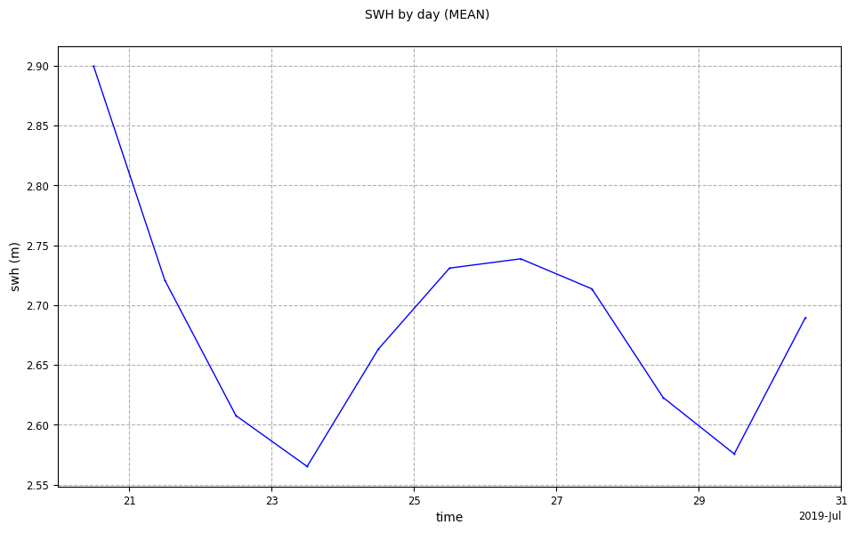
Temporal evolution of the SWH, averaged by day

[6]:

swh_day_plot = CasysPlot(data=ad, data_name="SWH by day", stat="mean")
swh_day_plot.show()

[6]:

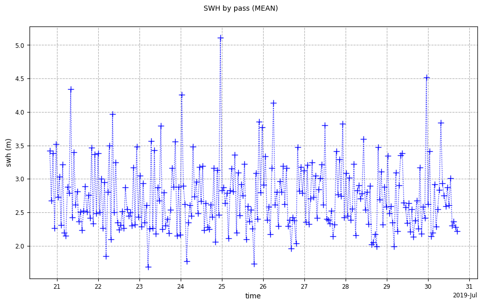
../_images/examples_example_basic_Temporal_Monitoring_12_0.png

Temporal evolution of the SWH, averaged by pass

[7]:

swh_pass_plot = CasysPlot(
    data=ad,
    data_name="SWH by pass",
    stat="mean",
    # We define some visualization parameters
    plot_params=PlotParams(line_style=":", marker_style="+", marker_size=8, grid=True),
)

swh_pass_plot.show()

[7]:

../_images/examples_example_basic_Temporal_Monitoring_14_0.png

To learn more about temporal diagnostic definition, please visit this documentation page.