Click here to download this notebook.

Geographical box statistic on mean SWH

[2]:

from casys.readers import CLSTableReader

from casys import CasysPlot, DataParams, DateHandler, Field, NadirData

NadirData.enable_loginfo()

Dataset definition

[3]:

# Reader definition
table_name = "TABLE_C_J3_B_GDRD"
start = DateHandler("2019-07-20 19:23")
end = DateHandler("2019-07-30 17:21")

reader = CLSTableReader(
    name=table_name,
    date_start=start,
    date_end=end,
    time="time",
    longitude="LONGITUDE",
    latitude="LATITUDE",
)

# Data container definition
ad = NadirData(source=reader)

var_swh = Field(name="swh", source="IIF(FLAG_VAL.ALTI == 0, SWH.ALTI, DV)", unit="m")

var_sel = Field(name="box_sel", source="IIF(FLAG_VAL.ALTI == 0, 1, DV)")

Definition of the statistic

The add_geobox_stat method allows to define geobox diagnostics.

Here we define a geobox statistic of the SWH variable, with mean and count computation.

[4]:

ad.add_geobox_stat(
    name="SWH geo box stat",
    field=var_swh,
    stats=["mean", "count"],
    res_lon=(-180, 180, 2),
    res_lat=(-90, 90, 2),
    # Limiting the count statistic to points validating var_sel
    box_selection=var_sel,
)

Compute

[5]:

ad.compute()

2025-05-14 11:03:41 INFO    Reading ['LONGITUDE', 'LATITUDE', 'swh', 'box_sel_312583c3-680f-4320-963c-4d6306aa6406']
2025-05-14 11:03:45 INFO    Computing diagnostics ['SWH geo box stat']
2025-05-14 11:03:45 INFO    Computing done.

Map plot

[6]:

swh_grid_plot = CasysPlot(data=ad, data_name="SWH geo box stat", stat="mean")
swh_grid_plot.show()

[6]:

../_images/examples_example_basic_Gridded_Map_10_0.png

[7]:

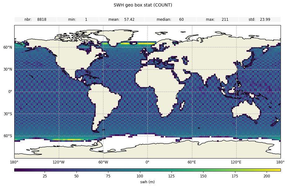
swh_grid_plot_c = CasysPlot(data=ad, data_name="SWH geo box stat", stat="count")
swh_grid_plot_c.add_stat_bar()
swh_grid_plot_c.show()

[7]:

../_images/examples_example_basic_Gridded_Map_11_0.png

3D plot

[8]:

swh_grid_plot_c = CasysPlot(
    data=ad,
    data_name="SWH geo box stat",
    stat="count",
    plot="3d",
    data_params=DataParams(x_limits=(-150, -100), y_limits=(-75, -25)),
)
swh_grid_plot_c.show()

[8]:

../_images/examples_example_basic_Gridded_Map_13_0.png

To learn more about geographical box diagnostic definition, please visit this documentation page.