


Investigation at regional scales of sea level variability at low and medium frequencies
L. Fenoglio-Marc (University of Technology Darmstadt, Germany), Y. Wang (Institute of Geodesy and Geophysics, China) and E. Groten (University of Technology Darmstadt, Germany)
Sea level variability at low and medium frequencies at regional scales and its mathematical representation in a model are investigated. The main areas of interest are the Mediterranean Sea, the North Sea and the Baltic Sea. The South China Sea is also considered.
The seasonal and interannual variability of monthly sea level anomalies (SLAs) and its relation to the variability of three atmospheric fields—sea surface temperature (STA), atmospheric pressure (APA) and wind speed (WSA) anomalies—are studied using spectral analysis methods and statistical techniques [Fenoglio-Marc, 1999]. Real and complex principal component analysis (PCA and CPCA) provide a compact description of the spatial and temporal variability of the data series, compressing the variability into a small number of statistical modes. Ordinary correlation methods and canonical correlation analysis (CCA) are applied to investigate the statistical relationships between the SLA and the other parameters. The SLA field corresponds to five years of TOPEX/POSEIDON (T/P) altimetry data, from October 1992 to September 1997. The corresponding APA and WSA fields are obtained from the T/P GDRs. The STA field corresponds to four years of data, from April 1992 to March 1996, computed from monthly ATSR ERS data.
European Seas
The spectral analysis method is applied to the data globally on each sea, as well as locally on a grid of points. The global spectral analysis of the T/P SLA field shows different spectral characteristics for the sea level height variability in the three seas. The corresponding Lomb normalized periodogram [Press et al., 1992] is given in Figure 1.
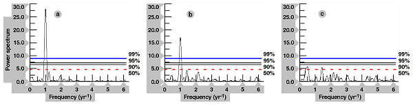
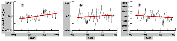
The annual frequency signal is particularly strong in the Mediterranean Sea. In both the Mediterranean Sea and the North Sea the power of the annual signal is above the 99% confidence level, while in the Baltic Sea the first two peaks of the spectrum have a lower confidence level, which is above 50%. The first dominant components have periods of about 360, 280 and 180 days in the Mediterranean Sea; 360, 240 and 720 days in the North Sea; and 720, 240 and 180 days in the Baltic Sea. A model for the sea level variability is computed using the first few spectral components identified by the spectral analysis. The long-term trend is estimated by least-squares fitting of the residuals after elimination of this model. The global analysis shows a trend of 7.1 ± 1.0 mm/yr in the Mediterranean Sea, 3.5 ± 3.0 mm/yr in the North Sea and –10.0 ± 7.6 mm/yr in the Baltic Sea (Figure 2).
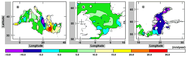
The local analysis shows that the dominant components and the trends are local. The higher trends observed in the Mediterranean Sea correspond to well-known oceanic circulation features: the largest positive trend occurs at the Ierapetra Gyre (28 mm/yr) and the largest high negative trend west of Greece (-15 mm/yr). In the North Sea the drift is lower (± 5 mm/yr) and in the Baltic Sea the drift has a north-south distribution: up to -15 mm/yr in the northern part and up to 5 mm/yr in the southern part (Figure 3). The error estimated for the trend is low in the Mediterranean and higher in the North Sea, and especially in the Baltic Sea, as in the global study. The trends are interpreted as interannual variability, due to the short time interval investigated. In the Mediterranean Sea, the results are in agreement with numerical simulations of the interannual variability of the upper ocean circulation [Pinardi et al., 1997]. Investigation of six years of T/P altimetry data, from October 1992 to September 1998, gives similar results except for the trend in the Baltic Sea, a region where the estimated error of the trend is large (+2 ± 7.0 mm/yr). A similar analysis is performed on the other atmospheric parameters.
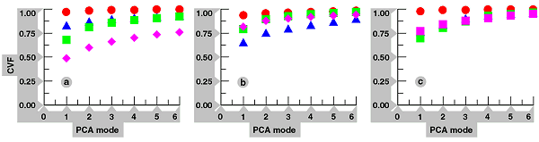
The PCA method identifies linear transformations of the dataset that concentrate as much variance as possible into a small number of variables [Preisendorfer, 1988], called statistical modes. The results shows that the total variance of the SLA field is contained in the first few modes in the Mediterranean Sea, while in the Baltic Sea, and in the North Sea in particular, several modes are necessary to explain the variance of the field. The first mode of the SLA field accounts for 83%, 65% and 77% respectively of the total variance in the Mediterranean Sea, North Sea and Baltic Sea. Figure 4 shows the cumulative fraction of total anomaly variance (CVF) accounted for by the first six statistical modes for the four fields. The PCA confirms the results obtained in the global and local analysis. In the Mediterranean Sea in particular the seasonal and interannual variabilities at regional scale are clearly identified in the spatial patterns of the first modes: the first spatial PCA pattern of SLA represents the rise and fall of the sea in the basin, the other modes show features of independent strong variability, such as the Alborean Gyre in the second mode and the interannual variability east of Greece in the third mode.
To investigate coupling between the SLA, STA, APA and WSA fields, a simple correlation method and two statistical methods—the direct SVD and the PCA-CCA methods—are used. These methods identify spatial and temporal patterns of coupled variability [Nicholls, 1986]. In the first statistical method, the pairs of patterns express as much as possible of the mean-squared temporal covariance between the two fields; in the second they have the maximum correlation coefficient. The relationship between the datasets is quantified by the cumulative squared covariance fraction (CSCF) in the direct SVD method and by the correlation coefficients between the expanded coefficients in the PCA-CCA method. The success of each model in compressing the data is quantified by the CVF. The fields are highly correlated if the CSCF, the CVF and the correlation coefficients are near to unity.
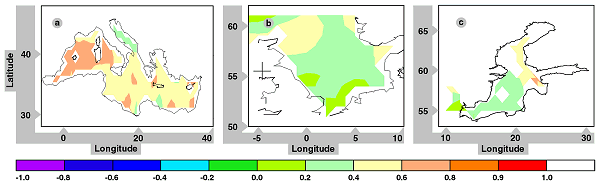
A significant correlation between the SLA and STA fields is found in the Mediterranean Sea, and between the SLA and WSA fields in the North Sea and the Baltic Sea, which partially explains the observed difference in the SLA patterns in the three seas. The homogeneous and the heterogeneous correlation maps are obtained by correlating the observed data and the expansion coefficient for a given mode, which correspond respectively to the same field and to the coupled field. The heterogeneous correlation maps of SLA and STA in the Mediterranean Sea and of SLA and WSA in the North Sea and in the Baltic Sea, corresponding to the first mode of the direct SVD method, are shown in Figure 5. They are quite similar to the simple correlation maps of the gridded data. This shows that the first mode of the models accounts for most of the coupled variability.
China Sea
The mean sea level slope over the China Sea was computed from the first five years of T/P data after removing the seasonal terms. A multivariate statistical technique is used to isolate and detect "quasi-oscillatory" components of the sea level variability. The most significant peaks are detected at a period of about 365 days, 180 days and 60 days above the 99% significance level. The rates of mean sea level variation over the China Sea are in the range of –1.8 mm/yr to +3.7 mm/yr, and +0.6 mm/yr on average, which indicates that the China Sea level rose slightly at an average rate of +0.5 mm/yr in the investigated period. Sea level variability derives from interactions between traveling waves of different spatial scales and temporal frequency. CPCA is a powerful technique that allows propagating features (standing oscillations and traveling waves) in the time and spatial domains to be detected and dissected in terms of their spatial and temporal behavior. The first CPCA eigenvector is shown in Figure 6a. A large cyclonic eddy centered at about 18°N, 118°E and with a radius of two degrees is clearly visible. This eddy was first identified in altimetric data from T/P in 1994 and verified by both a drifting buoy and the sea surface temperature [Soong et al., 1995]. The wavelet time-frequency spectrum analysis gives the eddy evolution , which has an annual period (Figure 6.b).
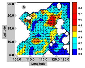
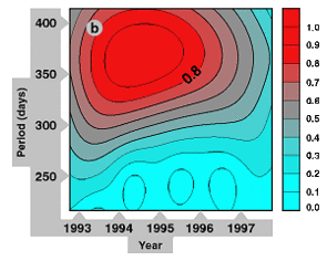
Figure 6: Amplitude and phase of the first CPCA eigenvector (a) and normalized wavelet time-frequency spectrum of the first CPCA (b) in the South China Sea.
Future research
Monitoring of long-term sea level variability requires altimetry data from various missions. Due to the higher accuracy of the T/P data, the variability model estimated using T/P data will be used as a reference in multi-satellite mission investigations.
References:
- Fenoglio-Marc, L., 1999: Variability at low and medium frequencies of sea level and atmospheric-oceanic parameters from dense coverage data in European Seas, Geophysical Journal International (submitted).
- Nicholls, N., 1987: The use of canonical correlation to study teleconnections, Monthly Weather Review, Vol. 115, pp.393-399.
- Pinardi, N., G. Korres, A. Lascaratos, V. Roussenov, E. Stanev, 1997: Numerical simulations of the interannual variability of the Mediterranean Sea upper ocean circulation, Geophysical Research Letters, Vol. 24, N.4, pp.425-428.
- Preisendorfer, R.W., 1988: Principal component analysis in Meteorology and Oceanography, Developments in the Atmospheric Science, 17, Elsevier Amsterdam
- Press W., S. Teukolsky, W. Vetterling, B. Flannery, 1992: Numerical Recipes in Fortran, second edition, Cambridge University Press
- Soong Y.S., J-H. Hu, C.R. Ho, P.P. Niiler, 1995: Cold core eddy detected in South China Sea, EOS 76, 345-347
News
 Archives .
- Aviso Newsletter .
- Newsletter 1 .
- Newsletter 2 .
- Newsletter 3 .
- Newsletter 4 .
- Newsletter 5 .
- Newsletter 6.
- Newsletter 7 .
- Jason-1, after T/P.
- Jason system overview and status.
- Ssalto, new ground segment.
- Review of 1999 and future AVISO activities.
- Jason-1 Calibration/Validation.
- Absolute altimeter calibration in Corsica.
- AVISO CALVAL Activities.
- Multi-variate assimilation to initialize El Niño predictions.
- Investigation at regional scales of sea level variability.
- Assimilating TOPEX/POSEIDON data to better understand Warm Pool replenishment and depletion.
- Further details of the 1997-98 El Niño.
- TOPEX/POSEIDON and TAO: Comparative simulation.
- Newsletter 8.
- Newsletter 9.
- Newsletter 10.
- Search.
- Front-page news.
- Image of the month .
- Operational news and status .